When you think about an invention of a new model for algorithmic trading, there are only three key elements you need to start your work with: creativity, data, and programming tool. Assuming that the last two are already in your possession, all what remains is seeking and finding a great new idea! With no offense, that’s the hardest part of the game.
To be successful in discovering new trading solutions you have to be completely open-minded, relaxed and full of spatial orientation with the information pertaining to your topic. Personally, after many years of programming and playing with the digital signal processing techniques, I have discovered that the most essential aspect of well grounded research is data itself. The more, literally, I starred at time-series changing their properties, the more I was able to capture subtle differences, often overlooked by myself before, and with the aid of intuition and scientific experience some new ideas simply popped up.
Here I would like to share with you a part of this process.
In one of the previous articles I outlined one of many possible ways of the FX time-series extraction from the very fine data sets. As a final product we have obtained two files, namely:
audusd.bid.1h
audusd.ask.1h
corresponding to Bid and Ask prices for Forex AUDUSD pair’s trading history between Jan 2000 and May 2010. Each file contained two columns of numbers: Time (Modified Julian Day) and Price. The time resolution has been selected to be 1 hour.
FOREX trading lasts from Monday to Friday, continuously for 24 hours. Therefore the data contain regular gaps corresponding to weekends. As the data coverage is more abundant comparing to, for example, much shorter trading windows of equities or ETFs around the world, that provides us with a better understanding of trading directions within every week time frame. Keeping that in mind, we might be interested in looking at directional information conveyed by the data as a seed of a potential new FX model.
As for now, let’s solely focus on initial pre-processing of Bid and Ask time-series and splitting each week into a common cell array.
% FX time-series analysis
% (c) Quant at Risk, 2012
%
% Part 1: Separation of the weeks

close all; clear all; clc;

% --analyzed FX pair
pair=['audusd'];

% --data
n=['./',pair,'/',pair];     % a common path to files
na=[n,'.ask.1h'];
nb=[n,'.bid.1h'];
d1=load(na); d2=load(na);   % loading data
d=(d1+d2)/2;                % blending
clear d1 d2
For a sake of simplicity, in line 16, we decided to use a simple average of Bid and Ask 1-hour prices for our further research. Next, we create a weekly template, $x$, for our data classification, and we find the total number of weeks available for analysis:
% time constraints from the data
t0=min(d(:,1));
tN=max(d(:,1));
t1=t0-1;

% weekly template for data classification
x=t1:7:tN+7;

% total number of weeks
nw=length(x)-1;

fprintf(upper(pair));
fprintf(' time-series: %3.0f weeks (%5.2f yrs)\n',nw,nw/52);
what in our case returns a positive information:
AUDUSD time-series: 539 weeks (10.37 yrs)
The core of programming exercise is to split all 539 weeks and save them into a cell array of $week$. As we will see in the code section below, for some reasons we may want to assure ourselves that each week will contain the same number of points, therefore any missing data from our FX data provider will be interpolated. To do that efficiently, we use the following function which makes use of Piecewise Cubic Hermite Interpolating Polynomial interpolation for filling gapped data point in the series:
function [x2,y2]=gapinterpol(x,y,dt);
    % specify axis
    x_min=x(1);
    x_max=x(length(x));
    x2=(x_min:dt:x_max);
    % inperpolate gaps
    y2=pchip(x,y,x2);
end
The separation of weeks we realize in our program by:
week={};  % an empty cell array
avdt=[];

for i=1:nw
    % split FX signal according to week
    [r,c,v]=find(d(:,1)>x(i) & d(:,1)<x(i+1));
    x1=d(r,1); y1=d(r,2);
    % interpolate gaps, use 1-hour bins
    dt=1/24;
    [x2,y2]=gapinterpol(x1,y1,dt);
    % check the average sampling time, should equal to dt
    s=0;
    for j=1:length(x2)-1
        s=s+(x2(j+1)-x2(j));
    end
    tmp=s/(length(x2)-1);
    avdt=[avdt; tmp];
    % store the week signal in a cell array
    tmp=[x2; y2]; tmp=tmp';
    week{i}=tmp;
end
fprintf('average sampling after interpolation = %10.7f [d]\n',max(avdt));
where as a check-up we get:
average sampling after interpolation = 0.0416667 [d]
what corresponds to the expected value of $1/24$ day with a sufficient approximation.
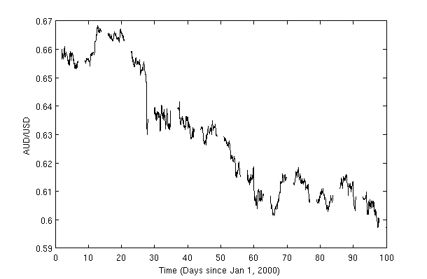
A quick visual verification of our signal processing,
scrsz = get(0,'ScreenSize');
h=figure('Position',[70 scrsz(4)/2 scrsz(3)/1.1 scrsz(4)/2],'Toolbar','none');
hold off;
for i=1:nw
    w=week{i};
    x=w(:,1); y=w(:,2);
    % plot weekly signal
    hold on; plot(x,y,'k');
end
xlim([0 100]);
uncovers our desired result:
Explore Further
→ Trading Forex: (2) Trend Identification
1 comment
Hi Pawel, I think that in line #15 you should use “d1=load(na); d2=load(nb);” instead of “na” in both cases.
Regards