It is one of the most fundamental approaches in measuring the risk, but truly worth revising its calculation. Value-at-Risk (VaR). A magical number quoted at the end of the day by the banks’ financial risk managers, portfolios’ risk managers, and risk managers simply concerned about the expected risk threshold not to be, hopefully, exceeded on the next day. What is so magical about it? According to definition, given a specific time horizon and taking into account last $N$ days of our trading activity, we can always calculate a number which would provide us with a simple answer to the question: if something really unexpected happened on the next day, what would be the loss margin we could for sure suffer? Well, welcome to the world of VaR!
More formally, given a daily (or, weekly, monthly, etc.) distribution of returns (of, for example, a single stock, a portfolio of assets, etc.), we are interested in finding the value of $VaR_\alpha$ of, say, $\alpha=0.05$ (five percent) which would say to as that there is 5% of chances that the value of $VaR_{0.05}$ would be exceeded in trading on the next day. This value is located in the left tail of the distribution and, by convention, it is given as positive number. Therefore, we define $VaR_\alpha$ as:
$$
P[X\le VaR_\alpha] = 1 – \alpha
$$ where $X$ is a random variable and can, as in our assumed case, represent a 1-day return on a traded asset or a portfolio of assets.
Beautiful! We have the risk threshold provided as a number. But in practice, how should we calculate $VaR_\alpha$? Here come into spotlight some of the shortcomings of VaR in general. VaR depends on the time-frame of the daily returns we examine: therefore $VaR_\alpha$ as a number will be different if you include last 252 trading days in estimation comparing to last 504 trading days (2 years). Intuitively, the more data (more days, years, etc.) we have the better estimation of $VaR_\alpha$, right? Yes and no. Keep in mind that the dynamic of the trading market changes continuously. In early 80s there was no high-frequency trading (HFT). It dominated trading traffic after the year of 2000 and now HFT plays a key role (an influential factor) in making impact on prices. So, it would be a bit unfair to compare $VaR_\alpha$ estimated in 80s with what is going on right now. $VaR_\alpha$ assumes that the distribution of returns is normal. Not most beautiful assumption but the most straightforward to compute $VaR_\alpha$. Should we use $VaR_\alpha$? Yes, but with caution.
Okay then, having $VaR_\alpha$ calculated we know how far the loss could reach at the $1-\alpha$ confidence level. The next super important question in risk management every risk manager should ask or at least be interested in reporting is: if $VaR_\alpha$ event occurs on the next day, what is the expected loss we might expect to suffer (say, in dollars)? $VaR_\alpha$ is the threshold. Now we are interested in the expected value of loss given the exceedance. It is the definition of expected shortfall and is based on the concept of conditional probability as follows:
$$
E[X\ |\ X>VaR_\alpha] = ES \ .
$$ In general, if our daily distribution of returns can be described by a function $f(x)$ which would represent a power density function (pdf), then:
$$
ES = \frac{1}{\alpha} \int_{-\infty}^{VaR_\alpha} xf(x)dx \ .
$$
Given any data set of returns, $R_t\ (t=1,…,N)$, calculated from our price history,
$$
R_t = \frac{P_{t+1}}{P_t} -1
$$ both numbers, $VaR_\alpha$ and $ES$ can be, in fact, calculated in two ways. The first method is based on the empirical distribution, i.e. using data as given:
$$
VaR_\alpha = h_i^{VaR} \ \ \mbox{for}\ \ \sum_{i=1}^{M-1} H_i(h_{i+1}-h_i) \le \alpha
$$ where $H$ represents the normalized histogram of $R_t$ (i.e., its integral is equal 1) and $M$ is the number of histograms bins. Similarly for $ES$, we get:
$$
ES = \sum_{i=1}^{h_i^{VaR}} h_iH_i(h_{i+1}-h_i) \ .
$$ The second method would be based on integrations given the best fit to the histogram of $R_t$ using $f(x)$ being a normal distribution. As we will see in the practical example below, both approaches returns different values, and an extra caution should be undertaken while reporting the final risk measures.
Case Study: IBM Daily Returns in 1987
The year of 1987 came into history as the most splendid time in the history of stock trading. Why? Simply because of so-called Black Monday on Oct 19, where markets denoted over 20% losses in a single trading day. Let’s analyse the case of daily returns and their distribution for IBM stock, as analysed by a risk manager after the close of the market on Thu, Dec 31, 1978. The risk manager is interested in the estimation of 1-day 95% VaR threshold, i.e. $VaR_0.05$, and the expected shortfall if on the next trading day (Jan 4, 1988) the exceedance event would occur. Therefore, let’s assume that our portfolio is composed solely of the IBM stock and we have the allocation of the capital of $C$ dollars in it as for Dec 31, 1987.
Using a record of historical trading, IBM.dat, of the form:
IBM
DATES 	      OPEN 	HIGH 	  LOW 	    CLOSE 	VOLUME
03-Jan-1984   0.000000 	0.000000  0.000000  30.437500 	0.000000
04-Jan-1984   0.000000 	0.000000  0.000000  30.968750 	0.000000
05-Jan-1984   0.000000 	0.000000  0.000000  31.062500 	0.000000
06-Jan-1984   0.000000 	0.000000  0.000000  30.875000 	0.000000
...
04-Mar-2011   0.000000 	0.000000  0.000000  161.830000 	0.000000
07-Mar-2011   0.000000 	0.000000  0.000000  159.930000 	0.000000
containing the close price of IBM stock, in Matlab, we extract the data for the year of 1987, then we construct a vector of daily returns $R_t$ on the stock,
% Reading in the data
fn=['IBM.dat'];
ftsD=ascii2fts(fn,1,2);
range=[datenum('02-Jan-1987'),datenum('31-Dec-1987')];
drr=[datestr(range(1)),'::',datestr(range(2))];
fts=ftsD(drr);
data=fts2mat(fts,1);

% R_t vector
rdata=data(2:end,5)./data(1:end-1,5)-1;

% Plotting
figure(1);
subplot(2,1,1);
plot(data(:,1)-datenum('2-Jan-1987'),data(:,5));
xlim([0 365]); ylabel('IBM Close Price ($)');
subplot(2,1,2);
plot(data(2:end,1)-datenum('2-Jan-1987'),rdata);
xlim([0 365]); ylabel('R_t')
xlabel('t (days)')
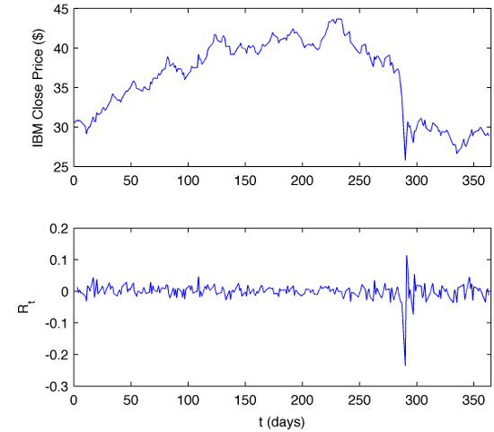
and present the data graphically:
Having our data, let’s find $VaR_{0.05}$ and corresponding $ES$,
% Construct the normalized histogram
[H,h]=hist(rdata,100);
hist(rdata,100);
sum=0;
for i=1:length(H)-1
    sum=sum+(H(i)*(h(i+1)-h(i)));
end
figure(2)
H=H/sum;
bar(h,H,'FaceColor',[0.7 0.7 0.7],'EdgeColor',[0.7 0.7 0.7])

% Calculate VaR 95 based on empirical distribution
sum=0;
i=1;
while (i<length(H))
    sum=sum+(H(i)*(h(i+1)-h(i)));
    if(sum>=0.05)
        break;
    end
    i=i+1;
end
VaR=h(i)
hold on; plot(h(i),0,'ro'); % mark VaR in the plot

% Fit the normal distribution to R_t data
[muhat,sigmahat] = normfit([rdata]');
Y = normpdf(h,muhat(1),sigmahat(1));
hold on; plot(h,Y,'b-'); % and plot the fit using blue line

% Find for the fitted N(muhat,sigmahat) VaR 95%
sum=0;
i=1;
while (i<length(h))
    sum=sum+(Y(i)*(h(i+1)-h(i)));
    if(sum>=0.05)
        break;
    end
    i=i+1;
end
VaR_fit=h(i)
hold on; plot(h(i),0,'ro','markerfacecolor','r'); % mark VaR_fit
ivar=i;

% Calculate the Expected Shortfall
%  based on fitted normal distribution
sum=0;
i=1;
while (i<=ivar)
    sum=sum+(h(i)*Y(i)*(h(i+1)-h(i)));
    i=i+1;
end
ES_fit=sum/0.05
hold on; plot(ES_fit,0,'ko','markerfacecolor','k');

% Add numbers to the plot
text(-0.23,25,['1-Day VaR and Expected Shortfall']);
text(-0.23,23.5,['as for 31/12/1987']);
text(-0.23,20,['VaR = ',num2str(VaR*-1,3),' (',num2str(VaR*-100,2),'%)']);
text(-0.23,18,['ES  = ',num2str(ES_fit*-1,3),' (',num2str(ES_fit*-100,2),'%)']);
text(-0.23,13,['\mu = ',num2str(muhat,2)]);
text(-0.23,11,['\sigma = ',num2str(sigmahat,2)]);
xlabel('R_t');
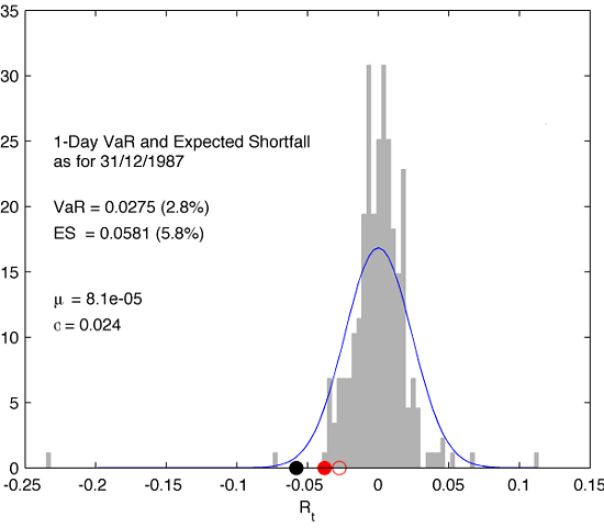
marking all numbers in resulting common plot:
In the plot, filled red and black markers correspond to $VaR_{0.05}$ and $ES$, respectively, and are calculated using the fitted normal distribution. Both values have been displayed in the plot as well. In addition to that, the plot contains a red open circle marker denoting the value of $VaR_{0.05}$ obtained from the empirical histogram discrete integration. Please note how the choice of the method influences the value of VaR.
The derived numbers tell the risk manager that in 95% of cases one should feel confident that the value of $VaR_{0.05}$ will not be exceed in trading of IBM on Jan 4, 1988 (next trading day). $C\times VaR_{0.05} = 0.028C$ would provide us with the loss amount (in dollars) if such undesired event had occurred. And if it was the case indeed, the expected loss (in dollars) we potentially would suffer, would be $C\times ES = 0.058C$.
Now it easy to understand why the Black Swan event of Oct 19, 1987 falls into the category of super least likely moves in the markets. It places itself in the far left tail of both empirical and fitted distributions denoting an impressive loss of 23.52% for IBM on that day. If we assume that the daily price changes are normally distributed then probability of a drop of at least 22 standard deviations is
$$
P(Z\le -22) = \Phi(-22) = 1.4 \times 10^{-107} \ .
$$ This is astronomically rare event!
They say that a lightening does not strike two times, but if a 1-day drop in the market of the same magnitude had occurred again on Jan 4, 1988, our long position in IBM would cause us to suffer not the loss of $0.058C$ dollars but approximately $0.23C$. Ahhhuc!

