Simulation of Portfolio Value using Geometric Brownian Motion Model

Having in mind the upcoming series of articles on building a backtesting engine for algo traded portfolios, today I decided to drop a short post on a simulation of the portfolio realised profit and loss (P&L). In the future I will use some results obtained below for a discussion of key statistics used in the evaluation of P&L at any time when it is required by the portfolio manager.

Assuming that we trade a portfolio of any assets, its P&L can be simulated in a number of ways. One of the quickest method is the application of geometric brownian motion (GBM) model with a drift in time of $\mu_t$ and the process standard deviation of $\sigma_t$ over its total time interval. The model takes its form as follows:
$$
dS_t = \mu_t S_t dt + \sigma_t S_t dz
$$ where $dz\sim N(0,dt)$ and the process has variance equal to $dt$ (the process is brownian). Let $t$ is the present time and the portfolio has an initial value of $S_t$ dollars. The target time is $T$ therefore portfolio time horizon of evaluation is $\tau=T-t$ at $N$ time steps. Since the GBM model assumes no correlations between the values of portfolio on two consecutive days (in general, over time), by integrating $dS/S$ over finite interval we get a discrete change of portfolio value:
$$
\Delta S_t = S_{t-1} (\mu_t\Delta t + \sigma_t\epsilon \sqrt{\Delta t}) \ .
$$ For simplicity, one can assume that both parameters of the model, $\mu_t$ and $\sigma_t$ are constant over time, and the random variable $\epsilon\sim N(0,1)$. In order to simulate the path of portfolio value, we go through $N$ iterations following the formula:
$$
S_{t+1} = S_t + S_t(\mu_t\Delta t + \sigma_t \epsilon_t \sqrt{\Delta t})
$$ where $\Delta t$ denotes a local volatility defined as $\sigma_t/\sqrt{N}$ and $t=1,…,N$.

Example

Let’s assume that initial portfolio value is $S_1=\$10,000$ and it is being traded over 252 days. We allow the underlying process to have a drift of $\mu_t=0.05$ and the overall volatility of $\sigma_t=5%$ constant over time. Since the simulation in every of 252 steps depends on $\epsilon$ drawn from the normal distribution $N(0,1)$, we can obtain any number of possible realisations of the simulated portfolio value path.

Coding quickly the above model in Matlab,

mu=0.05;      % drift
sigma=0.05;   % std dev over total inverval
S1=10000;     % initial capital ($)
N=252;        % number of time steps (trading days)
K=1;          % nubber of simulations

dt=sigma/sqrt(N);   % local volatility

St=[S1];
for k=1:K
    St=[S1];
    for i=2:N
        eps=randn; 
        S=St(i-1)+St(i-1)*(mu*dt+sigma*eps*sqrt(dt));
        St=[St; S];
    end
    hold on; plot(St);
end
xlim([1 N]);
xlabel('Trading Days')
ylabel('Simulated Portfolio Value ($)');

lead us to one of the possible process realisations,

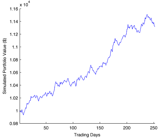
quite not too bad, with the annual rate of return of about 13%.

The visual inspection of the path suggests no major drawbacks and low volatility, therefore pretty good trading decisions made by portfolio manager or trading algorithm. Of course, the simulation does not tell us anything about the model, the strategy involved, etc. but the result we obtained is sufficient for further discussion on portfolio key metrics and VaR evolution.