GARCH(p,q) Model and Trade’s Exit Strategy

Forecasting future has always been a part of human untamed skill to posses. In an enjoyable Hollywood production of Next Nicolas Cage playing a character of Frank Cadillac has an ability to see the future just up to a few minutes ahead. This allows him to take almost immediate actions to avoid the risks. Now, just imagine for a moment that you are an (algorithmic) intraday trader. What would you offer for a glimpse of knowing what is going to happen within following couple of minutes? What sort of risk would you undertake? Is it really possible to deduce the next move on your trading chessboard?

Most probably the best answer to this question is: it is partially possible. Why then partially? Well, even with a help of mathematics and statistics, obviously God didn’t want us to know future by putting his fingerprint into our equations and calling it a random variable. Smart, isn’t it? Therefore, our goal is to work harder in order to guess what is going to happen next!?

In this post I will shortly describe one of the most popular methods of forecasting future volatility in financial time-series employing a GARCH model. Next, I will make use of 5-min intraday stock data of close prices to show how to infer possible stock value in next 5 minutes using current levels of volatility in intraday trading. Ultimately, I will discuss an exit strategy from a trade based on forecasted worst case scenario (stock price is forecasted to exceed the assumed stop-loss level). But first, let’s warm up with some cute equations we cannot live without.

Inferring Volatility

Capturing and digesting volatility is somehow like an art that does not attempt to represent external, recognizable reality but seeks to achieve its effect using shapes, forms, colors, and textures. The basic idea we want to describe here is a volatility $\sigma_t$ of a random variable (rv) of, e.g. an asset price, on day $t$ as estimated at the end of the previous day $t-1$. How to do it in the most easiest way? It’s simple. First let’s assume that a logarithmic rate of change of the asset price between two time steps is:
$$
r_{t-1} = \ln\frac{P_{t-1}}{P_{t-2}}
$$ what corresponds to the return expressed in percents as $R_{t-1}=100[\exp(r_{t-1})-1]$ and we will be using this transformation throughout the rest of the text. This notation leaves us with a window of opportunity to denote $r_t$ as an innovation to the rate of return under condition that we are able, somehow, to deduce, infer, and forecast a future asset price of $P_t$.

Using classical definition of a sample variance, we are allowed to write it down as:
$$
\sigma_t^2 = \frac{1}{m-1} \sum_{i=1}^{m} (r_{t-i}-\langle r \rangle)^2
$$ what is our forecast of the variance rate in next time step $t$ based on past $m$ data points, and $\langle r \rangle=m^{-1}\sum_{i=1}^{m} r_{t-i}$ is a sample mean. Now, if we examine return series which is sampled every one day, or an hour, or a minute, it is worth to notice that $\langle r \rangle$ is very small as compared with the standard deviation of changes. This observation pushes us a bit further in rewriting the estimation of $\sigma_t$ as:
$$
\sigma_t^2 = \frac{1}{m} \sum_{i=1}^{m} r_{t-i}^2
$$ where $m-1$ has been replaced with $m$ by adding an extra degree of freedom (equivalent to a maximum likelihood estimate). What is superbly important about this formula is the fact that it gives an equal weighting of unity to every value of $r_{t-i}$ as we can always imagine that quantity multiplied by one. But in practice, we may have a small wish to associate some weights $\alpha_i$ as follows:
$$
\sigma_t^2 = \sum_{i=1}^{m} \alpha_i r_{t-i}^2
$$ where $\sum_{i=1}^{m} \alpha_i = 1$ what replaces a factor of $m^{-1}$ in the previous formula. If you think for a second about the idea of $\alpha$’s it is pretty straightforward to understand that every observation of $r_{t-i}$ has some significant contribution to the overall value of $\sigma_t^2$. In particular, if we select $\alpha_i<\alpha_j$ for $i>j$, every past observation from the most current time of $t-1$ contributes less and less.

In 1982 R. Engle proposed a tiny extension of discussed formula, finalized in the form of AutoRegressive Conditional Heteroscedasticity ARCH($m$) model:
$$
\sigma_t^2 = \omega + \sum_{i=1}^{m} \alpha_i r_{t-i}^2
$$ where $\omega$ is the weighted long-run variance taking its position with a weight of $\gamma$, such $\omega=\gamma V$ and now $\gamma+\sum_{i=1}^{m} \alpha_i = 1$. What the ARCH model allows is the estimation of future volatility, $\sigma_t$, taking into account only past $m$ weighted rates of return $\alpha_i r_{t-i}$ and additional parameter of $\omega$. In practice, we aim at finding weights of $\alpha_i$ and $\gamma$ using maximum likelihood method for given return series of $\{r_i\}$. This approach, in general, requires approximately $m>3$ in order to describe $\sigma_t^2$ efficiently. So, the question emerges: can we do much better? And the answer is: of course.

Four years later, in 1986, a new player entered the ring. His name was Mr T (Bollerslev) and he literally crushed Engle in the second round with an innovation of the Generalized AutoRegressive Conditional Heteroscedasticity GARCH($p,q$) model:
$$
\sigma_t^2 = \omega + \sum_{i=1}^{p} \alpha_i r_{t-i}^2 + \sum_{j=1}^{q} \beta_j \sigma_{t-j}^2
$$ which derives its $\sigma_t^2$ based on $p$ past observations of $r^2$ and $q$ most recent estimates of the variance rate. The inferred return is then equal $r_t=\sigma_t\epsilon_t$ where $\epsilon_t\sim N(0,1)$ what leave us with a rather pale and wry face as we know what in practice that truly means! A some sort of simplification meeting a wide applause in financial hassle delivers the solution of GARCH(1,1) model:
$$
\sigma_t^2 = \omega + \alpha r_{t-1}^2 + \beta \sigma_{t-1}^2
$$ which derives its value based solely on the most recent update of $r$ and $\sigma$. If we think for a shorter while, GARCH(1,1) should provide us with a good taste of forecasted volatility when the series of past couple of returns were similar, however its weakness emerges in the moments of sudden jumps (shocks) in price changes what causes overestimated volatility predictions. Well, no model is perfect.

Similarly as in case of ARCH model, for GARCH(1,1) we may use the maximum likelihood method to find the best estimates of $\alpha$ and $\beta$ parameters leading us to a long-run volatility of $[\omega/(1-\alpha-\beta)]^{1/2}$. It is usually achieved in the iterative process by looking for the maximum value of the sum among all sums computed as follows:
$$
\sum_{i=3}^{N} \left[ -\ln(\sigma_i^2) – \frac{r_i^2}{\sigma_i^2} \right] $$ where $N$ denotes the length of the return series $\{r_j\}$ ($j=2,…,N$) available for us. There are special dedicated algorithms for doing that and, as we will see later on, we will make use of one of them in Matlab.

For the remaining discussion on verification procedure of GARCH model as a tool to explain volatility in the return time-series, pros and cons, and other comparisons of GARCH to other ARCH-derivatives I refer you to the immortal and infamous quant’s bible of John Hull and more in-depth textbook by a financial time-series role model Ruey Tsay.

Predicting the Unpredictable

The concept of predicting the next move in asset price based on GARCH model appears to be thrilling and exciting. The only worry we may have, and as it has been already recognized by us, is the fact that the forecasted return value is $r_t=\sigma_t\epsilon_t$ with $\epsilon_t$ to be a rv drawn from a normal distribution of $N(0,1)$. That implies $r_t$ to be a rv such $r_t\sim N(0,\sigma_t)$. This model we are allowed to extend further to an attractive form of:
$$
r_t = \mu + \sigma_t\epsilon_t \ \ \ \sim N(\mu,\sigma_t)
$$ where by $\mu$ we will understand a simple mean over past $k$ data points:
$$
\mu = k^{-1} \sum_{i=1}^{k} r_{t-i} \ .
$$ Since we rather expect $\mu$ to be very small, its inclusion provides us with an offset in $r_t$ value modeling. Okay, so what does it mean for us? A huge uncertainty in guessing where we gonna end up in a next time step. The greater value of $\sigma_t$ inferred from GARCH model, the wider spread in possible values that $r_t$ will take. God’s fingerprint. End of hopes. Well, not exactly.

Let’s look at the bright side of our $N(\mu,\sigma_t)$ distribution. Remember, never give in too quickly! Look for opportunities! Always! So, the distribution has two tails. We know very well what is concealed in its left tail. It’s the devil’s playground of worst losses! Can a bad thing be a good thing? Yes! But how? It’s simple. We can always compute, for example, 5% quantile of $Q$, what would correspond to finding a value of a rv $r_t$ for which there is 5% and less of chances that the actual value of $r_t$ will be smaller or equal $Q$ (a sort of equivalent of finding VaR). Having this opportunity, we may wish to design a test statistic as follows:
$$
d = Q + r’
$$ where $r’$ would represent a cumulative return of an open trading position. If you are an intraday (or algorithmic high-frequency) trader and you have a fixed stop-loss limit of $s$ set for every trade you enter, a simple verification of a logical outcome of the condition of:
$$
d < s \ ? $$ provides you immediately with an attractive model for your decision to close your position in next time step based on GARCH forecasting derived at time $t-1$. All right, let’s cut the cheese and let’s see now how does that work in practice!

5-min Trading with GARCH Exit Strategy

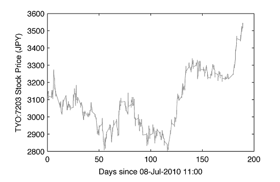
In order to illustrate the whole theory of GARCH approach and dancing at the edge of uncertainty of the future, we analyze the intraday 5-min stock data of Toyota Motor Corporation traded at Toyota Stock Exchange with a ticker of TYO:7203. The data file of TYO7203m5.dat contains a historical record of trading in the following form:

TYO7203
DATES      TIMES OPEN HIGH LOW  CLOSE VOLUME
07/8/2010  11:00 3135 3140 3130 3130  50900
07/8/2010  11:05 3130 3135 3130 3130  16100
07/8/2010  11:10 3130 3145 3130 3140  163700
...
01/13/2011 16:50 3535 3540 3535 3535  148000
01/13/2011 16:55 3540 3545 3535 3535  1010900

i.e. it is spanned between 8-Jul-2010 11:00 and 13-Jan-2011 16:55. Using Matlab language,

% Forecasting Volatility, Returns and VaR for Intraday 
%   and High-Frequency Traders
%
% (c) 2013 QuantAtRisk.com, by Pawel Lachowicz

clear all; close all; clc;

%% ---DATA READING AND PREPROCESSING

fname=['TYO7203m5.dat'];
% construct FTS object for 5-min data
fts=ascii2fts(fname,'T',1,2,[1 2]);
% sampling
dt=5; % minutes

% extract close prices
cp=fts2mat(fts.CLOSE,1);

% plot 5-min close prices for entire data set
figure(1);
plot(cp(:,1)-cp(1,1),cp(:,2),'Color',[0.6 0.6 0.6]);
xlabel('Days since 08-Jul-2010 11:00');
ylabel('TYO:7203 Stock Price (JPY)');

let’s plot 5-min close prices for a whole data set available:

Now, a moment of concentration. Let’s imagine you are trading this stock based on 5-min close price data points. It is late morning of 3-Dec-2010, you just finished your second cup of cappuccino and a ham-and-cheese sandwich when at 10:55 your trading model sends a signal to open a new long position in TYO:7203 at 11:00.

% ---DATES SPECIFICATION

% data begin on/at
date1='08-Jul-2010';
time1='11:00';
% last available data point (used for GARCH model feeding)
dateG='03-Dec-2010';
timeG='12:35';
% a corresponding data index for that time point (idxGARCH)
[idxGARCH,~,~]=find(cp(:,1)==datenum([dateG,' ' ,timeG]));
% enter (trade) long position on 03-Dec-2010 at 11:00am
dateT='03-Dec-2010';
timeT='11:00';
% a corresposding data index for that time point(idx)
[idx,~,~]=find(cp(:,1)==datenum([dateT,' ',timeT]));

You buy $X$ shares at $P_{\rm{open}}=3310$ JPY per share at 11:00 and you wait observing the asset price every 5 min. The price goes first up, than starts to fall down. You look at your watch, it is already 12:35. Following a trading data processing, which your Matlab does for you every 5 minutes,

 % ---DATA PREPROCESSING (2)

% extract FTS object spanned between the beginning of data
%  and last available data point
ftsGARCH=fetch(fts,date1,time1,dateG,timeG,1,'d');
cpG=fts2mat(ftsGARCH.CLOSE,1); % extract close prices (vector)
retG=log(cpG(2:end,2)./cpG(1:end-1,2)); % extract log return (vector)

figure(1); 
hold on; 
plot(cp(1:idxGARCH,1)-cp(1,1),cp(1:idxGARCH,2),'b') % a blue line in Figure 2

figure(2);
% plot close prices
x=1:5:size(cpG,1)*5;
x=x-x(idx+1); % 
plot(x,cpG(:,2),'-ok');
xlim([-20 110]);
ylim([3285 3330]);
ylabel('TYO:7203 Stock Price (JPY)'); 
xlabel('Minutes since 03-Dec-2010 11:00');
% add markers to the plot
hold on; %
plot(-dt,cpG(idx,2),'o','MarkerEdgeColor','g');
hold on; 
plot(0,cpG(idx+1,2),'o','MarkerFaceColor','k','MarkerEdgeColor','k');
% mark -0.5% stoploss line
xs=0:5:110;
stoploss=(1-0.005)*3315; % (JPY)
ys=stoploss*ones(1,length(xs));
plot(xs,ys,':r');

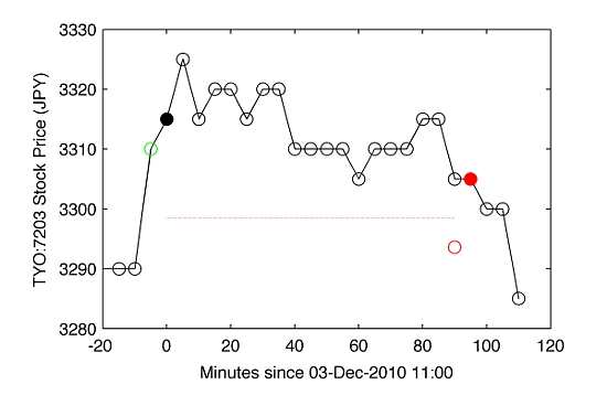
you re-plot charts, here: as for data extracted at 3-Dec-2010 12:35,

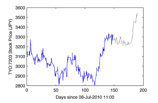
where by blue line it has been marked the current available price history of the stock (please ignore a grey line as it refers to the future prices which we of course don’t know on 3-Dec-2010 12:35 but we use it here to understand better the data feeding process in time, used next in GARCH modeling), and

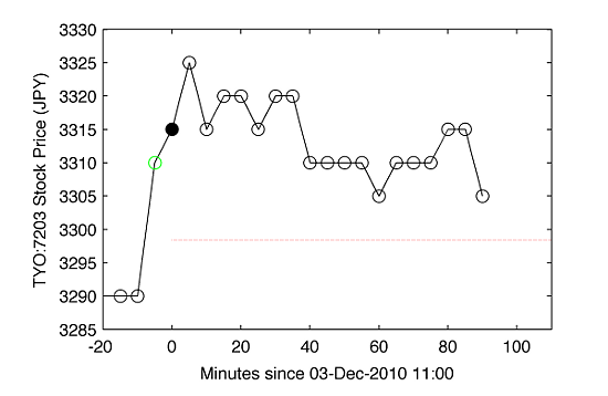
what presents the price history with time axis adjusted to start at 0 when a trade has been entered (black filled marker) as suggested by the model 5 min earlier (green marker). Assuming that in our trading we have a fixed stop-loss level of -0.5% per every single trade, the red dotted line in the figure marks the corresponding stock price of suggested exit action. As for 12:35, the actual trading price of TYO:7203 is still above the stop-loss. Great! Well, are you sure?

As we trade the stock since 11:00 every 5 min we recalculate GARCH model based on the total data available being updated by a new innovation in price series. Therefore, as for 12:35, our GARCH modeling in Matlab,

% ---ANALYSIS

% GARCH(p,q) parameter estimation
model = garch(3,3) % define model
[fit,VarCov,LogL,Par] = estimate(model,retG)
% extract model parameters
parC=Par.X(1) % omega
parG=Par.X(2) % beta (GARCH)
parA=Par.X(3) % alpha (ARCH)
% estimate unconditional volatility
gamma=1-parA-parG
VL=parC/gamma;
volL=sqrt(VL)
% redefine model with estimatated parameters
model=garch('Constant',parC,'GARCH',parG,'ARCH',parA)

% infer 5-min varinace based on GARCH model
sig2=infer(model,retG); % vector

runs,

model = 
    GARCH(3,3) Conditional Variance Model:
    --------------------------------------  
    Distribution: Name = 'Gaussian'
               P: 3
               Q: 3
        Constant: NaN
           GARCH: {NaN NaN NaN} at Lags [1 2 3]
            ARCH: {NaN NaN NaN} at Lags [1 2 3]
____________________________________________________________
   Diagnostic Information

Number of variables: 7

Functions 
Objective:                            @(X)OBJ.nLogLikeGaussian(X,V,E,Lags,...)
Gradient:                             finite-differencing
Hessian:                              finite-differencing (or Quasi-Newton)

Constraints
Nonlinear constraints:                do not exist
 
Number of linear inequality constraints:    1
Number of linear equality constraints:      0
Number of lower bound constraints:          7
Number of upper bound constraints:          7

Algorithm selected
   sequential quadratic programming
____________________________________________________________
   End diagnostic information
                                                          Norm of First-order
 Iter F-count            f(x) Feasibility  Steplength        step  optimality
    0       8   -2.545544e+04   0.000e+00                           1.392e+09
    1      60   -2.545544e+04   0.000e+00   8.812e-09   8.813e-07   1.000e+02

Local minimum found that satisfies the constraints.

Optimization completed because the objective function is non-decreasing in 
feasible directions, to within the selected value of the function tolerance,
and constraints are satisfied to within the selected value of the constraint tolerance.

and returns the best estimates of GARCH model’s parameters:

   GARCH(1,1) Conditional Variance Model:
    ----------------------------------------
    Conditional Probability Distribution: Gaussian

                                  Standard          t     
     Parameter       Value          Error       Statistic 
    -----------   -----------   ------------   -----------
     Constant    2.39895e-07   6.87508e-08        3.48934
     GARCH{1}            0.9     0.0224136        40.1542
      ARCH{1}           0.05     0.0037863        13.2055

fit = 
    GARCH(1,1) Conditional Variance Model:
    --------------------------------------  
    Distribution: Name = 'Gaussian'
               P: 1
               Q: 1
        Constant: 2.39895e-07
           GARCH: {0.9} at Lags [1]
            ARCH: {0.05} at Lags [1]

defining the GARCH(1,1) model on 3-Dec-2010 12:35 of TYO:7302 as follows:
$$
\sigma_t^2 = 2.39895\times 10^{-7} + 0.05r_{t-1}^2 + 0.9\sigma_{t-1}^2 \ \ .
$$ where the long-run volatility $V=0.0022$ ($0.2\%$) at $\gamma=0.05$. Please note, that due to some computational mind tricks, we allowed to define the raw template of GARCH model as GARCH(3,3) which has been adjusted by Matlab’s solver down to resulting GARCH(1,1).

Based on the model and data available till $t-1=$ 12:35, we get a forecast of $\sigma_t$ value at $t=$ 12:40 to be

% forcast varianace 1-step (5-min) ahead, sigma^2_t
sig2_t=forecast(model,1,'Y0',retG,'V0',sig2); % scalar
sig_t=sqrt(sig2_t) % scalar

$$
\sigma_t=0.002 \ (0.2\%) \ .
$$
Plotting return series for our trade, at 12:35 we have:

% update a plot of 5-min returns
figure(3);
x=1:length(retG); x=x-idx; x=x*5;
plot(x,100*(exp(retG)-1),'ko-');  
xlim([-20 110]);
ylim([-0.8 0.8]);
xlabel('Minutes since 03-Dec-2010 11:00');
ylabel('R_t [%]');

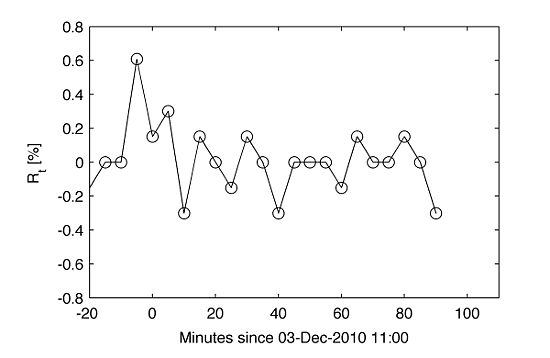
Estimating the mean value of return series by taking into account last 12 data points (60 min),

% estimate mean return over passing hour (dt*12=60 min)
mu=mean(retG(end-12:end))

we get $\mu=-2.324\times 10^{-4}$ (log values), what allows us to define the model for return at $t=$ 12:40 to be:
$$
R_t = \mu + \sigma_t\epsilon_t = -0.02324 + 0.2\epsilon \ , \ \ \ \epsilon\sim N(0,1)\ .
$$ The beauty of God’s fingerprint denoted by $\epsilon$ we can understand better but running a simple Monte-Carlo simulation and drawing 1000 rvs of $r_t=\mu+\sigma_t\epsilon$ which illustrate 1000 possible values of stock return as predicted by GARCH model!

% simulate 1000 rvs ~ N(0,sig_t)
r_t=sig_t*randn(1000,1);

One of them could be the one at 12:40 but we don’t know which one?! However, as discussed in Section 2 of this article, we find 5% quantile of $Q$ from the simulation and we mark this value by red filled circle in the plot.

tmp=[(length(retG)-idx)*5+5*ones(length(r_t),1) 100*(exp(r_t)-1)];
hold on; plot(tmp(:,1),tmp(:,2),'x');

Q=norminv(0.05,mu,sig_t); 
Q=100*(exp(Q)-1);

hold on; plot((length(retG)-idx)*5+5,Q,'or','MarkerFaceColor','r');

Including 1000 possibilities (blue markers) of realisation of $r_t$, the updated Figure 4 now looks like:

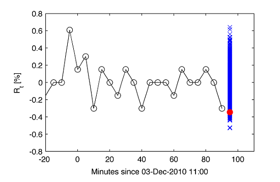
where we find from simulation $Q=-0.3447\%$. The current P&L for an open long position in TYO:7203,

% current P/L for the trade
P_open=3315; % JPY (3-Dec-2010 11:00)
cumRT=100*(cpG(end,2)/P_open-1) %  = r'

returns $r’=-0.3017\%$. Employing a proposed test statistic of $d$,

% test statistics (percent)
d=cumRT+Q

we get $d=r’+Q = -0.6464\%$ which, for the first time since the opening the position at 11:00, exceeds our stop-loss of $s=-0.5\%$. Therefore, based on GARCH(1,1) forecast and logical condition of $d\lt s$ to be true, our risk management engine sends out at 12:35 an order to close the position at 12:40. The forecasted closing price,

% forecasted stock price under test (in JPY)
f=P_open*(1+d/100)

is estimated to be equal 3293.6 JPY, i.e. -0.6464% loss.

At 12:40 the order is executed at 3305 JPY per share, i.e. with realized loss of -0.3017%.

The very last question you asks yourself is: using above GARCH Exit Strategy was luck in my favor or not? In other words, has the algorithm taken the right decision or not? We can find out about that only letting a time to flow. As you come back from the super-quick lunch break, you sit down, look at the recent chart of TYO:7203 at 12:55,

and you feel relief, as the price went further down making the algo’s decision a right decision.

For reference, the red filled marker has been used to denote the price at which we closed our long position with a loss of -0.3017% at 12:40, and by open red circle the forecasted price under $d$-statistics as derived at 12:35 has been marked in addition for the completeness of the grand picture and idea standing behind this post.

Jump Deeper

GARCH(1,1) Model in Python
Volatile Vol-of-Vol: How is Volatility of Volatility calculated?