Yahoo! Stock Data in Matlab and a Model for Dividend Backtesting

Within the evolution of Mathworks’ MATLAB programming environment, finally, in the most recent version labelled 2013a we received a longly awaited line-command facilitation for pulling stock data directly from the Yahoo! servers. What does that mean for quants and algo traders? Honestly, a lot. Now, simply writing a few commands we can have nearly all what we want. However, please keep in mind that Yahoo! data are free therefore not always in one hundred percent their precision remains at the level of the same quality as, e.g. downloaded from Bloomberg resources. Anyway, just for pure backtesting of your models, this step introduces a big leap in dealing with daily stock data. As usual, we have a possibility of getting open, high, low, close, adjusted close prices of stocks supplemented with traded volume and the dates plus values of dividends.

In this post I present a short example how one can retrieve the data of SPY (tracking the performance of S&P500 index) using Yahoo! data in a new Matlab 2013a and I show a simple code how one can test the time period of buying-holding-and-selling SPY (or any other stock paying dividends) to make a profit every time.

The beauty of Yahoo! new feature in Matlab 2013a has been fully described in the official article of Request data from Yahoo! data servers where you can find all details required to build the code into your Matlab programs.

Model for Dividends

It is a well known opinion (based on many years of market observations) that one may expect the drop of stock price within a short timeframe (e.g. a few days) after the day when the stock’s dividends have been announced. And probably every quant, sooner or later, is tempted to verify that hypothesis. It’s your homework. However, today, let’s look at a bit differently defined problem based on the omni-working reversed rule: what goes down, must go up. Let’s consider an exchange traded fund of SPDR S&P 500 ETF Trust labelled in NYSE as SPY.

First, let’s pull out the Yahoo! data of adjusted Close prices of SPY from Jan 1, 2009 up to Aug 27, 2013

% Yahoo! Stock Data in Matlab and a Model for Dividend Backtesting
% (c) 2013 QuantAtRisk.com, by Pawel Lachowicz

close all; clear all; clc;

date_from=datenum('Jan 1 2009');
date_to=datenum('Aug 27 2013');

stock='SPY';

adjClose = fetch(yahoo,stock,'adj close',date_from,date_to);
div = fetch(yahoo,stock,date_from,date_to,'v')
returns=(adjClose(2:end,2)./adjClose(1:end-1,2)-1);

% plot adjusted Close price of  and mark days when dividends
% have been announced
plot(adjClose(:,1),adjClose(:,2),'color',[0.6 0.6 0.6])
hold on;
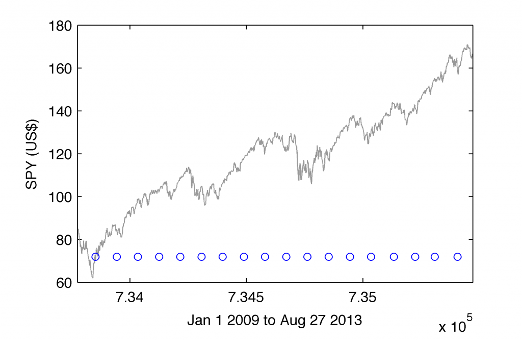
plot(div(:,1),min(adjClose(:,2))+10,'ob');
ylabel('SPY (US$)');
xlabel('Jan 1 2009 to Aug 27 2013');

and visualize them:

Having the data ready for backtesting, let’s look for the most profitable period of time of buying-holding-and-selling SPY assuming that we buy SPY one day after the dividends have been announced (at the market price), and we hold for $dt$ days (here, tested to be between 1 and 40 trading days).

% find the most profitable period of holding SPY (long position)
neg=[];
for dt=1:40

buy=[]; sell=[];
for i=1:size(div,1)
    % find the dates when the dividends have been announced
    [r,c,v]=find(adjClose(:,1)==div(i,1));
    % mark the corresponding SPY price with blue circle marker
    hold on; plot(adjClose(r,1),adjClose(r,2),'ob');
    % assume you buy long SPY next day at the market price (close price)
    buy=[buy; adjClose(r-1,1) adjClose(r-1,2)];
    % assume you sell SPY in 'dt' days after you bought SPY at the market
    % price (close price)
    sell=[sell; adjClose(r-1-dt,1) adjClose(r-1-dt,2)];
end

% calculate profit-and-loss of each trade (excluding transaction costs)
PnL=sell(:,2)./buy(:,2)-1;
% summarize the results
neg=[neg; dt sum(PnL<0) sum(PnL<0)/length(PnL)];

end

If we now sort the results according to the percentage of negative returns (column 3 of neg matrix), we will be able to get:

>> sortrows(neg,3)

ans =
   18.0000    2.0000    0.1111
   17.0000    3.0000    0.1667
   19.0000    3.0000    0.1667
   24.0000    3.0000    0.1667
    9.0000    4.0000    0.2222
   14.0000    4.0000    0.2222
   20.0000    4.0000    0.2222
   21.0000    4.0000    0.2222
   23.0000    4.0000    0.2222
   25.0000    4.0000    0.2222
   28.0000    4.0000    0.2222
   29.0000    4.0000    0.2222
   13.0000    5.0000    0.2778
   15.0000    5.0000    0.2778
   16.0000    5.0000    0.2778
   22.0000    5.0000    0.2778
   27.0000    5.0000    0.2778
   30.0000    5.0000    0.2778
   31.0000    5.0000    0.2778
   33.0000    5.0000    0.2778
   34.0000    5.0000    0.2778
   35.0000    5.0000    0.2778
   36.0000    5.0000    0.2778
    6.0000    6.0000    0.3333
    8.0000    6.0000    0.3333
   10.0000    6.0000    0.3333
   11.0000    6.0000    0.3333
   12.0000    6.0000    0.3333
   26.0000    6.0000    0.3333
   32.0000    6.0000    0.3333
   37.0000    6.0000    0.3333
   38.0000    6.0000    0.3333
   39.0000    6.0000    0.3333
   40.0000    6.0000    0.3333
    5.0000    7.0000    0.3889
    7.0000    7.0000    0.3889
    1.0000    9.0000    0.5000
    2.0000    9.0000    0.5000
    3.0000    9.0000    0.5000
    4.0000    9.0000    0.5000

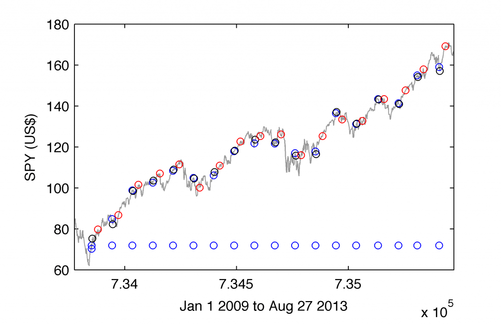
what simply indicates at the most optimal period of holding the long position in SPY equal 18 days. We can mark all trades (18 day holding period) in the chart:

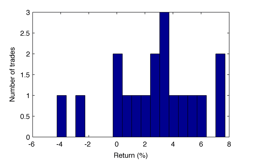
where the trade open and close prices (according to our model described above) have been marked in the plot by black and red circle markers, respectively. Only 2 out of 18 trades (PnL matrix) occurred to be negative with the loss of 2.63% and 4.26%. The complete distribution of profit and losses from all trades can be obtained in the following way:

figure(2);
hist(PnL*100,length(PnL))
ylabel('Number of trades')
xlabel('Return (%)')

returning

Let’s make some money!

The above Matlab code delivers a simple application of the newest build-in connectivity with Yahoo! server and the ability to download the stock data of our interest. We have tested the optimal holding period for SPY since the beginning of 2009 till now (global uptrend). The same code can be easily used and/or modified for verification of any period and any stock for which the dividends had been released in the past. Fairly simple approach, though not too frequent in trading, provides us with some extra idea how we can beat the market assuming that the future is going to be/remain more or less the same as the past. So, let’s make some money!