Information Ratio and its Relative Strength for Portfolio Managers

The risk and return are the two most significant quantities investigated within the investment performance. We expect the return to be highest at the minimum risk. In practice, a set of various combinations is always achieved depending on a number of factors related to the investment strategies and market behaviours, respectively. The portfolio manager or investment analyst is interested in the application of most relevant tool in order to described the overall performance. The arsenal is rich but we need to know the character of outcomes we wish to underline prior to fetching the proper instruments from the workshop.

In general there are two schools of investment performance. The first one is strictly related to the analysis of time-series on the tick-by-tick basis. All I mean by tick is a time scale of your data, e.g. minutes or months. The analyst is concerned about changes in investments and risk tracked continuously. A good example of this sort of approach is measurement of Value-at-Risk and Expected Shortfall, Below Target Risk or higher-moments of Coskewness and Cokurtosis. It all supplements the n-Asset Portfolio Construction with Efficient Frontier diagnostic.

The second school in the investment analysis is a macro-perspective. It includes the computation on $n$-period rolling median returns (or corresponding quantities), preferably annualized for the sake of comparison. This approach carries more meaning behind the lines rather than a pure tick time-series analysis. For the former, we track a sliding changes in accumulation and performance while for the latter we focus more closely on tick-by-tick risks and returns. For the sake of global picture and performance (market-oriented vantage point), a rolling investigation of risk and return reveals mutual tracking factors between different considered scenarios.

In this article I scratch the surface of the benchmark-oriented analysis with a special focus on the Information Ratio (IR) as an investment performance-related measure. Based on the market data, I test the IR in action and introduce a new supplementary measure of Information Ratio Relative Strength working as a second dimension for IR results.

1. Benchmark-oriented Analysis

Let’s assume you a portfolio manager and you manage over last 10 years 11 investment strategies. Each strategy is different, corresponds to different markets, style of investing, and asset allocation. You wish to get a macro-picture how well your investment performed and are they beating the benchmark. You collect a set of 120 monthly returns for each investment strategy plus their benchmarks. The easiest way to kick off the comparison process is the calculation of $n$-period median (or mean) returns.

Annualized Returns

The rolling $n$Y ($n$-Year) median return is defined as:
$$
\mbox{rR}_{j}(n\mbox{Y}) = \left[ \prod_{i=1}^{12n} (r_{i,j}+1)^{1/n} \right] -1
\ \ \ \ \ \mbox{for}\ \ \ j=12n,…,N\ \ (\mbox{at}\ \Delta j =1)
$$
where $r$ are the monthly median returns meeting the initial data selection criteria (if any) and $N$ denotes the total number of data available (in our case, $N=120$).

Any pre-selection (pre-filtering) of the input data becomes more insightful when contrasted with the benchmark performance. Thereinafter, by the benchmark we can assume a relative measure we will refer to (e.g. S\&P500 Index for US stocks, etc.) calculated as the rolling $n$Y median. Therefore, for instance, the 1Y (rolling) returns can be compared against the corresponding benchmark (index). The selection of a good/proper benchmark belongs to us.

Active Returns

We define active returns on the monthly basis as the difference between actual returns and benchmark returns,
$$
a_i = r_i – b_i ,
$$
as available at $i$ where $i$ denotes a continuous counting of months over past 120 months.

Annualized Tracking Risk (Tracking Error)

We assume the widely accepted definition of the tracking risk as the standard deviation of the active returns. For the sake of comparison, we transform it the form of the annualized tracking risk in the following way:
$$
\mbox{TR}_{j}(n\mbox{Y}) = \sqrt{12} \times \sqrt{ \frac{1}{12n-1} \sum_{i=1}^{12n} \left( a_{i,j}-\langle a_{i,j} \rangle \right)^2 }
$$
where the square root of 12 secures a proper normalization between calculations and $j=12n,…,N$.

Annualized Information Ratio (IR)

The information ratio is often referred to as a variation or generalised version of Sharpe ratio. It tells us how much excess return ($a_i$) is generated from the amount of excess risk taken relative to the benchmark. We calculate the annualized information ratio by dividing the annualised active returns by the annualised tracking risk as follows:
$$
\mbox{IR}_j(n\mbox{Y}) = \frac{ \left[ \prod_{i=1}^{12n} (a_{i,j}+1)^{1/n} \right] -1 } { TR_j(n\mbox{Y}) }
\ \ \ \ \ \mbox{for}\ \ \ j=12n,…,N
$$

We assume the following definition of the investment under-performance and out-performance, $P$, as defined based on IR:
$$
P_j =
\begin{cases}
P_j^{-} =\mbox{under-performance}, & \text{if } \mbox{IR}_j(n\mbox{Y}) \le 0 \\
P_j^{+} =\mbox{out-performance}, & \text{if } \mbox{IR}_j(n\mbox{Y}) > 0 .
\end{cases}
$$

Information Ratio Relative Strength of Performance

Since $P_j$ marks in time only those periods of time (months) where a given quantity under investigation achieved better results than the benchmark or not, it does not tell us anything about the importance (weight; strength) of this under/over-performance. The case could be, for instance, to observe the out-performance for 65\% of time over 10 years but barely beating the benchmark in the same period. Therefore, we introduce an additional measure, namely, the IR relative strength defined as:
$$
\mbox{IRS} = \frac{ \int P^{+} dt } { \left| \int P^{-} dt \right| } .
$$
The IRS measures the area under $\mbox{IR}_j(n\mbox{Y})$ function when $\mbox{IR}_j(n\mbox{Y})$ is positive (out-performance) relative to the area cofined between $\mbox{IR}_j(n\mbox{Y})$ function and $\mbox{IR}_j(n\mbox{Y})=0$. Thanks to that measure, we are able to estimate the revelance of
$$
\frac { n(P^{+}) } { n(P^{-}) + n(P^{+}) }
$$
ratio, i.e. the fraction of time when the examined quantity displayed out-performance over specified period of time (e.g. 10 years of data within our analysis). Here, $n(P^{+})$ counts number of $P_j^{+}$ instances.

2. Case Study

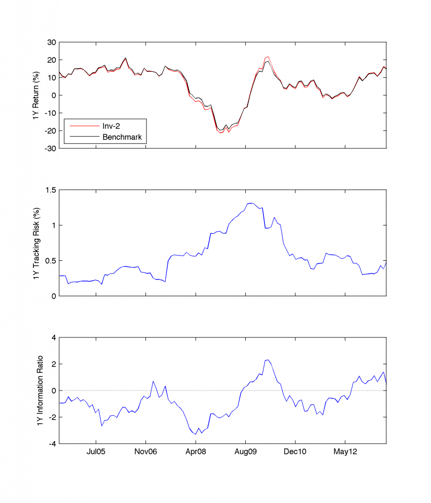
Let’s demonstrate the aforementioned theory in practice. Making use of real data, we perform a benchmark-oriented analysis for all 11 investment strategies. We derive 1Y rolling median returns supplemented by the correspoding 1Y tracking risk and information ratio measures. The following figure presents the results for 1Y returns of for the Balanced Options:

Interestingly to notice, the Investment Strategy-2 (Inv-2) displays an increasing tracking risk between mid-2007 and mid-2009 corresponding to the Credit Global Financial Crisis (GFC). This consistent surge in TR is explained by worse than average performance of the individual options, most probably dictated by higher than expected volatility of assets within portfolio. The 1Y returns of Inv-2 were able to beat the benchmark over only 25% of time, i.e. about 2.25 years since Jun/30 2004. We derive that conclusion based on the quantitative inspection of the Information Ratio plot (bottom panel).

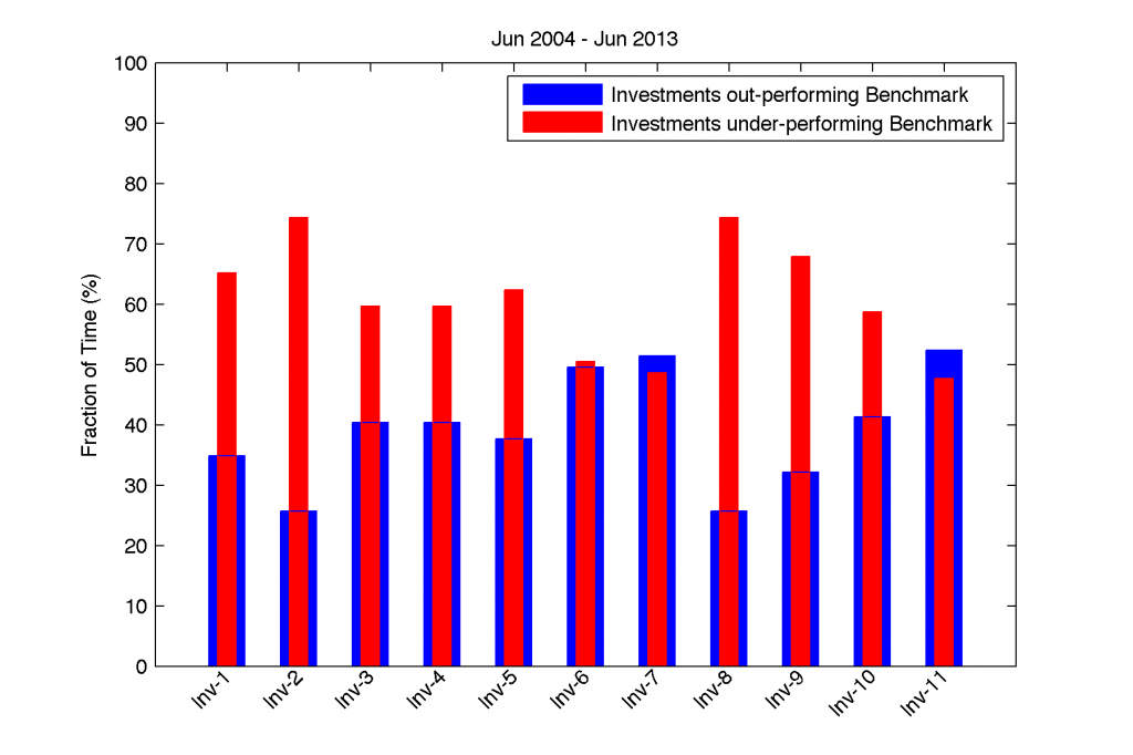
In order to understand the overall performance for all eleven investment strategies, we allow ourselves to compute the under-performance and out-performance ratios,
$$
\frac { n(P^{-}) } { n(P^{-}) + n(P^{+}) } \ \ \ \mbox{and} \ \ \ \frac { n(P^{+}) } { n(P^{-}) + n(P^{+}) } ,
$$
and plot these ratios in red and blue colour in the following figure, respectively:

Only two investment strategies, Inv-7 and Inv-11, managed to keep the out-performance time longer than their under-performance. Inv-8 denoted the highest ratio of under-performance to out-performance but also Inv-2 (consider above)performed equally badly.

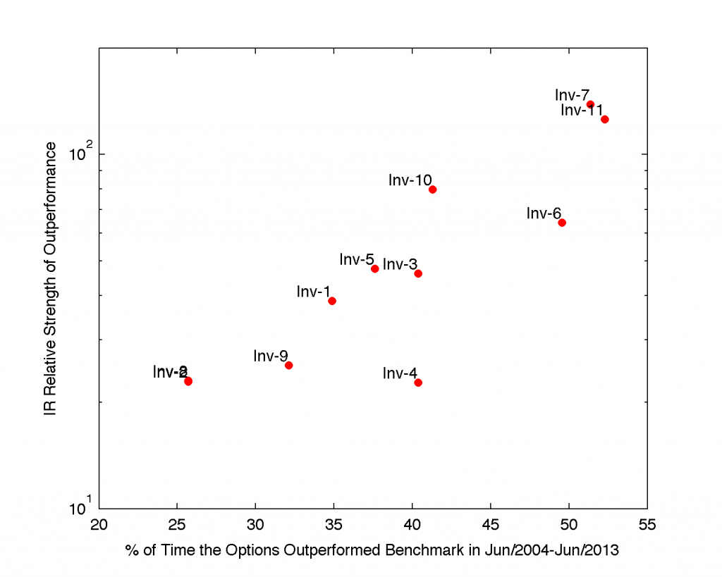
The 3rd dimension to this picture delivers the investigation of the IR Relative Strength measure for all investment strategies. We derive and display the results in next figure:

The plot reveals close-to-linear correlation between two considered quantities. Inv-7 and Inv-11 strategies confirm their relative strength of out-performance while Inv-2 and Inv-8 their weakness in delivering strong returns over their short period of out-performance.

It is of great interest to compare Inv-3, Inv-4, and Inv-10 strategies. While relative strength of out-performance of Inv-4 remains lower as contrasted with the latter ones (and can be explained by low volatility within this sort of investment strategy), Inv-10 denotes much firmer gains over benchmark than Inv-3 despite the fact that their out-performance period was nearly the same ($\sim$40%). Only the additional cross-correlation of IR Relative Strength outcomes as a function of the average return year-over-year is able to address the drivers of this observed relation.