There is only one goal in algorithmic stock trading: to win the game. To emerge victorious. To feel the sunlight again after the months of walking through the valley of shadows being stuck in the depths of algo drawdowns. An endless quest for the most brilliant minds, to find the way to win over and over, and over again. To discover a perfect solution as your new private weapon in this battleground. Is it possible? If the answer were so simple, we wouldn’t be so engaged in seeking for a golden mean.
However, algo trading is a journey, and sometimes in the process of programming and testing of our trading systems, we need to have an ideal trading model ready-to-use straight away! What I mean by the ideal model is a sort of template, a benchmark that will allow us to list a number of successful trades, their starting and closing times, open and close price of the trades being executed, and the realized return coming down to our pocket from each trade. Such a trading model template also allows us to look at the trading data from a different perspective and re-consider and/or apply an additional risk management framework. In fact, the benefits are limitless for the backtesting purposes.
In this post we will explore one of the easiest ways in programming a perfect model by re-directing the time-axis backwards. Using an example of the data of a Google, Inc. (GOOG) stock listed at NASDAQ, we will analyse the stock trading history and find all possible trades returning at least 3% over past decade.
The results of this strategy I will use within the upcoming (this week!) series of new posts on Portfolio Optimization in Matlab for Algo Traders.
Stock Trading Model and Data
Let’s imagine we are interested in finding a large number of trades with the expected return from each trade to be at least 3%. We consider GOOG stock (daily close prices) with data spanning 365$\times$10 days back in time since the present day (last 10 years). We will make use of Google Finance data powered by Quandl as described in one of my previous posts, namely, Create a Portfolio of Stocks based on Google Finance Data fed by Quandl. Shall we begin?
% Ideal Stock Trading Model for the Purpose of Backtesting Only
%
% (c) 2013 QuantAtRisk.com, by Pawel Lachowicz


clear all; close all; clc;

stocklist={'GOOG'};

% Read in the list of tickers and internal code from Quandl.com
[ndata, text, alldata] = xlsread('QuandlStockCodeListUS.xlsx');
quandlc=text(:,1); % again, as a list in a cell array
quandlcode=text(:,3) % corresponding Quandl's Price Code

% fetch stock data for last 10 years
date2=datestr(today,'yyyy-mm-dd')     % from
date1=datestr(today-365*10,'yyyy-mm-dd') % to

stockd={};
for i=1:length(stocklist)
    for j=1:length(quandlc)
        if(strcmp(stocklist{i},quandlc{j}))
            fprintf('%4.0f %s\n',i,quandlc{j});
            % fetch the data of the stock from Quandl
            % using recommanded Quandl's command and
            % saving them directly into FTS object (fts)
            fts=0;
            [fts,headers]=Quandl.get(quandlcode{j},'type','fints', ...
                          'authcode','ENTER_YOUR_CODE',...
                          'start_date',date1,'end_date',date2);
            stockd{i}=fts; % entire FTS object in an array's cell
        end
    end
end
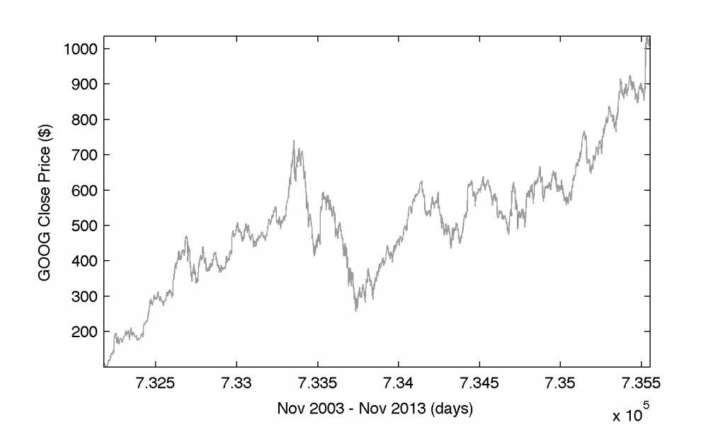
The extracted data of GOOG from Google Finance via Quandl we can visualize immediately as follows:
% plot the close prices of GOOG
cp=fts2mat(stockd{1}.Close,1);
plot(cp(:,1),cp(:,2),'color',[0.6 0.6 0.6])
xlim([min(cp(:,1)) max(cp(:,1))]);
ylim([min(cp(:,2)) max(cp(:,2))]);
xlabel('Nov 2003 - Nov 2013 (days)');
ylabel('GOOG Close Price ($)');
We open the trade on the first day (long position) and as time goes by, on the following day we check whether the stock value increased by 3% or more. If not, we increase the current time position by one day and check again. If the condition is met, we close the opened trade on the following trading (business) day at the stock’s market price. We allow to open a new trade at the stock’s market price one next business day after the day when the previous trade has been closed (exercised). Additionally, we check if the ‘running’ return from the open trade exceeds -5%. If so, we substitute the open time of a new trade with the time when the latter condition has been fulfilled (the same for the open price of that trade). The latter strategy allow us to restart the backtesting process therefore the search for a new profitable trade.
t0=cp(1,1);    % starting day for backtesting
tN=cp(end,1);  % last day

trades=[]; % open a log-book for all executed traded
status=0; % status meaning: 0-no open trade, 1-open trade
t=t0;
% we loop over time (t) [days]
while(t<tN)
    [r,~,~]=find(t==cp(:,1)); % check the row in cp vector
    if(~isempty(r))
       if(~status)
           topen=t; % time when we open the trade
           popen=cp(r,2); % assuming market price of the stock
           status=1;
       else
           ptmp=cp(r,2); % running close price
           rtmp=ptmp/popen-1; % running return of the open trade
           if(rtmp>0.03) % check 3% profit condition
               % if met, then
               tclose=busdate(t,1); % close time of the trade
                                    %  assumed on the next business day
               t=busdate(tclose,1); % next day in the loop
               if(tclose<=tN)
                   [r,~,~]=find(tclose==cp(:,1));
                   pclose=cp(r,2); % close price
                   ret=pclose/popen-1; % realized profit/loss
                   % save the trade details into log-book
                   trades=[trades; topen tclose popen pclose ret*100];
                   status=0; % change status of trading to not-open
                   % mark the opening of the trade as blue dot marker
                   hold on; plot(topen,popen,'b.','markerfacecolor','b');
                   % mark the end time of the trade
                   hold on; plot(tclose,pclose,'r.','markerfacecolor','r');
               end
           elseif(rtmp<=-0.05) % check an additional condition
               topen=t; % overwrite the time
               popen=cp(r,2); % and the price
               status=1; % sustain the status of the trade as 'open'
           else
               t=t+1;
           end
       end
    else
        t=t+1;
    end
end
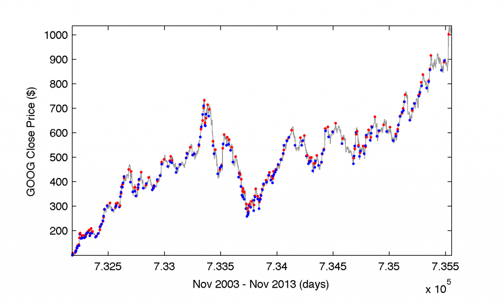
In this piece of code, in the variable matrix of trades (a log-book of all exercised trades) we store the history of all successful trades meeting our earlier assumed criteria. The only uncertainty that we allow to slip into our perfect solution is the one related to an instance when the the close price on the next business day occurs to be lower, generating the realized profit from the trade less than 3%. By plotting all good trades with the ending day of $tN$ set as for Nov 18, 2013, we get a messy picture:
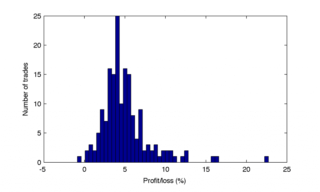
which translates into more intuitive one once we examine the distribution of profits from all trades:
figure(3);
hist(trades(:,5),50);
xlabel('Profit/loss (%)');
ylabel('Number of trades');
In this point the most valuable information is contained in the log-book which content we can analyze trade by trade:
>> format shortg
>> trades

trades =

   7.3218e+05   7.3218e+05       100.34        109.4       9.0293
   7.3218e+05   7.3220e+05       104.87          112       6.7989
   7.3221e+05   7.3221e+05       113.97       119.36       4.7293
   7.3221e+05   7.3222e+05       117.84       131.08       11.236
   7.3222e+05   7.3222e+05        129.6       138.37        6.767
   7.3223e+05   7.3224e+05       137.08       144.11       5.1284
   7.3224e+05   7.3224e+05       140.49       172.43       22.735
   7.3224e+05   7.3225e+05        187.4       190.64       1.7289
   ...
   7.3533e+05   7.3535e+05       783.05       813.45       3.8823
   7.3535e+05   7.3536e+05        809.1       861.55       6.4825
   7.3536e+05   7.3537e+05       857.23       915.89        6.843
   7.3546e+05   7.3549e+05       856.91       888.67       3.7063
   7.3549e+05   7.3553e+05       896.19       1003.3       11.952
where the columns correspond to the open and close time of the trade (a continuous Matlab’s time measure for the financial time-series; see datestr command for getting yyyy-mm-dd date format), open and close price of GOOG stock, and realized profit/loss of the trade, respectively.


