Walsh–Hadamard Transform and Tests for Randomness of Financial Return-Series

Randomness. A magic that happens behind the scene. An incomprehensible little blackbox that does the job for us. Quants. Many use it every day without thinking, without considering how those beautifully uniformly distributed numbers are drawn?! Why so fast? Why so random? Is randomness a byproduct of chaos and order tamed somehow? How trustful can we be placing this, of minor importance, command of random() as piece of our codes?

Randomness Built-in. Not only that’s a name of a chapter in my latest book but the main reason I’m writing this article: wandering sideways around the subject that led me to new undiscovered territories! In general the output in a form of a random number comes for a dedicated function. To be perfectly honest, it is like a refined gentleman, of sophisticated quality recognised by its efficiency when a great number of drafts is requested. The numbers are not truly random. They are pseudo-random. That means the devil resides in details. A typical pseudo-random number generator (PRNG) is designed for speed but defined by underlying algorithm. In most of computer languages Mersenne Twister developed by 松本 眞 and 西村 拓士 in 1997 has become a standard. As one might suspect, an algorithm must repeat itself and in case of our Japanese hero, its period is superbly long, i.e. $2^{19937}-1$. A reliable implementation in C or C++ guarantees enormous speedups in pseudo-random numbers generation. Interestingly, Mersenne Twister is not perfect. Its use had been discouraged when it comes to obtaining cryptographic random numbers. Can you imagine that?! But that’s another story. Ideal for a book chapter indeed!

In this post, I dare to present the very first, meaningful, and practical application of the Walsh–Hadamard Transform (WHT) in quantitative finance. Remarkably, this tool, of marginal use in digital signal processing, had been shown to serve as a great facility in testing any binary sequence for its statistically significant randomness!

Within the following sections we introduce the transform to finance. After Oprina et al. (2009) we encode WHT Significance Tests to Python (see Download section) and verify a hypothesis of the evidence of randomness as generated by Mersenne Twister PRNG against the alternative one at vey high significance levels of $\alpha\le 0.00001$. Next, we show a practical application of the WHT framework in search for randomness in any financial time-series by example of 30-min FX return-series and compare them to the results obtained from PRNG available in Python by default. Curious about the findings? Welcome to the world of magic!

1. Walsh–Hadamard Transform And Binary Sequences

I wish I had for You this great opening story on how Jacques Hadamard and Joseph L. Walsh teamed up with Jack Daniels on one Friday’s night in the corner pub somewhere in San Francisco coming up to a memorable breakthrough in theory of numbers. I wish I had! Well, not this time. However, as a make-up, below I will present in a nutshell a theoretical part on WHT I’ve been studying for past three weeks and found it truly mind-blowing because of its simplicity.

Let’s consider any real-valued discrete signal $X(t_i)$ where $i=0,1,…,N-1$. Its trimmed version, $x(t_i)$, of the total length of $n=2^M$ such that $2^M\le(N-1)$ and $M\in\mathbb{Z}^+$ at $M\ge 2$ is considered as an input signal for the Walsh–Hadamard Transform, the latter defined as:
$$
WHT_n = \mathbf{x} \bigotimes_{i=1}^M \mathbf{H_2}
$$ where the Hadamard matrix of order $n=2^M$ is obtainable recursively by the formula:
$$
\mathbf{H_{2^M}} =
\begin{pmatrix}
H_{2^{M-1}} & H_{2^{M-1}} \\
H_{2^{M-1}} & -H_{2^{M-1}}
\end{pmatrix}
\ \ \ \ \ \text{therefore} \ \ \ \ \ \mathbf{H_2} =
\begin{pmatrix}
1 & 1 \\
1 & -1
\end{pmatrix}
$$ and $\otimes$ denotes the Kronecker product between two matrices. Given that, $WHT_n$ is the dot product between the signal (1D array; vector) and resultant Kronecker multiplications of $\mathbf{H_2}$ $M$-times (Johnson & Puschel 2000).

1.1. Walsh Functions

The Walsh-Hadamard transform uses the orthogonal square-wave functions, $w_j(x)$, introduced by Walsh (1923), which have only two values $\pm 1$ in the interval $0\le x\lt 1$ and the value zero elsewhere. The original definition of the Walsh functions is based on the following recursive equations:
$$
w_{2j}(x) = w_j(2x)+(-1)^j w_j (2x -1) \quad \mbox{for} \ \ j=1,2,… w_{2j-1}(x) =
$$
$$
= w_{j-1}(2x)-(-1)^{j-1}
$$
$$
w_{j-1} (2x -1) \quad \mbox{for} \ \ j=1,2,…
$$ with the initial condition of $w_0(x)= 1$. You can meet with different ordering of Walsh functions in the literature but in general it corresponds to the ordering of the orthogonal harmonic functions $h_j(x)$, which are defined as:
$$
h_{2j}(x) = \cos(2\pi j x)\quad \mbox{for} \ \ j=0,1,… \\
h_{2j-1}(x) = \sin(2\pi j x)\quad \mbox{for} \ \ j=1,2,…
$$ on the interval $0\le x\lt 1$, and have zero value for all other values of $x$ outside this interval. A comparison of both function classes looks as follows:

where the first eight harmonic functions and Walsh functions are given in the left and right panels, respectively. Walsh functions with even and odd orders are called the cal and sal functions, respectively, and they correspond to the cosine and sine functions in Fourier analysis (Aittokallio et al. 2001).

1.2. From Hadamard to Walsh Matrix

In Python the Hadamard matrix of order $2^M$ is obtainable as a NumPy 2D array making use of SciPy module as follows:

from scipy.linalg import hadamard
M=3; n=2**M
H=hadamard(n)
print(H)

what is this case returns:

[[ 1  1  1  1  1  1  1  1]
 [ 1 -1  1 -1  1 -1  1 -1]
 [ 1  1 -1 -1  1  1 -1 -1]
 [ 1 -1 -1  1  1 -1 -1  1]
 [ 1  1  1  1 -1 -1 -1 -1]
 [ 1 -1  1 -1 -1  1 -1  1]
 [ 1  1 -1 -1 -1 -1  1  1]
 [ 1 -1 -1  1 -1  1  1 -1]]

Each row of the matrix corresponds to Walsh function. However, the ordering is different (Hadamard ordering). Therefore, to be able to “see” the shape of Walsh functions as presented in the figure above, we need to rearrange their indexing. The resultant matrix is known as Walsh matrix. We derive it in Python:

def Hadamard2Walsh(n):
    # Function computes both Hadamard and Walsh Matrices of n=2^M order
    # (c) 2015 QuantAtRisk.com, coded by Pawel Lachowicz, adopted after
    # au.mathworks.com/help/signal/examples/discrete-walsh-hadamard-transform.html
    import numpy as np
    from scipy.linalg import hadamard
    from math import log

    hadamardMatrix=hadamard(n)
    HadIdx = np.arange(n)
    M = log(n,2)+1

    for i in HadIdx:
        s=format(i, '#032b')
        s=s[::-1]; s=s[:-2]; s=list(s)
        x=[int(x) for x in s]
        x=np.array(x)
        if(i==0):
            binHadIdx=x
        else:
            binHadIdx=np.vstack((binHadIdx,x))

    binSeqIdx = np.zeros((n,M)).T

    for k in reversed(xrange(1,int(M))):
        tmp=np.bitwise_xor(binHadIdx.T[k],binHadIdx.T[k-1])
        binSeqIdx[k]=tmp

    tmp=np.power(2,np.arange(M)[::-1])
    tmp=tmp.T
    SeqIdx = np.dot(binSeqIdx.T,tmp)

    j=1
    for i in SeqIdx:
        if(j==1):
            walshMatrix=hadamardMatrix[i]
        else:
            walshMatrix=np.vstack((walshMatrix,hadamardMatrix[i]))
        j+=1

    return (hadamardMatrix,walshMatrix)

Therefore, by calling the function in an exemplary main program:

from WalshHadamard import Hadamard2Walsh
import matplotlib.pyplot as plt
import numpy as np

M=3; n=2**M
(H,W)=Hadamard2Walsh(n)
# display Hadamard matrix followed by Walsh matrix (n=8)
print(H); print;
print(W)

# a visual comparison of Walsh function (j=2)
M=3;
n=2**M
_,W=Hadamard2Walsh(n)
plt.subplot(2,1,1)
plt.step(np.arange(n).tolist(),W[2],where="post")
plt.xlim(0,n)
plt.ylim(-1.1,1.1); plt.ylabel("order M=3")

M=8;
n=2**M
_,W=Hadamard2Walsh(n)
plt.subplot(2,1,2)
plt.step(np.arange(n).tolist(),W[2],where="post")
plt.xlim(0,n)
plt.ylim(-1.1,1.1); plt.ylabel("order M=8")

plt.show()

first, we display Hadamard and Walsh matrices of order $n=2^3$, respectively:

[[ 1  1  1  1  1  1  1  1]
 [ 1 -1  1 -1  1 -1  1 -1]
 [ 1  1 -1 -1  1  1 -1 -1]
 [ 1 -1 -1  1  1 -1 -1  1]
 [ 1  1  1  1 -1 -1 -1 -1]
 [ 1 -1  1 -1 -1  1 -1  1]
 [ 1  1 -1 -1 -1 -1  1  1]
 [ 1 -1 -1  1 -1  1  1 -1]]

[[ 1  1  1  1  1  1  1  1]
 [ 1  1  1  1 -1 -1 -1 -1]
 [ 1  1 -1 -1 -1 -1  1  1]
 [ 1  1 -1 -1  1  1 -1 -1]
 [ 1 -1 -1  1  1 -1 -1  1]
 [ 1 -1 -1  1 -1  1  1 -1]
 [ 1 -1  1 -1 -1  1 -1  1]
 [ 1 -1  1 -1  1 -1  1 -1]]

and next we visually verify that the shape of the third Walsh function ($j=2$) is preserved for two different orders, here $M=3$ and $M=8$, respectively:

The third possibility of ordering the Walsh functions is so that they are arranged in increasing order of their sequencies or number of zero-crossings: sequency order. However, we won’t be interested in it this time.

1.3. Signal Transformations

As we have seen in the beginning, the WHT is able to perform a signal transformation for any real-vauled time-series. The sole requirement is that the signal ought to be of $2^M$ length. Now, it should be obvious why is so. When you think about WHT for a longer second you may understand its uniqueness as contrasted with the Fourier transform. Firstly, the waveforms are much simpler. Secondly, the complexity of computation is significantly reduced. Finally, if the input signal is converted from its original form down to only two discrete values $\pm 1$, we end up with a bunch of trivial arithmetical calculations while WHT.

The Walsh-Hadamard transform found its application in medical signal processing, audio/sound processing, signal and image compression, pattern recognition, and cryptography. In the most simplistic cases, one deals with the input signal to be of the binary form, e.g. 01001011010110. If we consider the binary function $f: \mathbb{Z}_2^n \rightarrow \mathbb{Z}_2$ then the following transformation is possible:
$$
\bar{f}(\mathbf{x}) = 1 – 2f(\mathbf{x}) = (-1)^{f(\mathbf{x})}
$$ therefore $\bar{f}: \mathbb{Z}_2^n \rightarrow \{-1,1\}$. What does it do is it performs the following conversion, for instance:
$$
\{0,1,0,1,1,0,1,0,0,0,1,…\} \rightarrow \{-1,1,-1,1,1,-1,1,-1,-1,-1,1,…\}
$$ of the initial binary time-series. However, what would be more interesting for us as it comes to the financial return-series processing, is the transformation:
$$
\bar{f}(\mathbf{x}) = \left\{
\begin{array}{l l}
1 & \ \text{if $f(\mathbf{x})\ge 0$}\\
-1 & \ \text{if $f(\mathbf{x})\lt 0$}
\end{array} \right.
$$ Given that, any return-series in the value interval $[-1,1]$ (real-valued) is transformed to the binary form of $\pm 1$, for example:
$$
\{0.031,0.002,-0.018,-0.025,0.011,…\} \rightarrow \{1,1,-1,-1,1,…\} \ .
$$ This simple signal transformation in connection with the power of Walsh-Hadamard Transform opens new possibilities of analysing the underlying true signal. WHT is all “made of” $\pm 1$ values sleeping in its Hadamard matrices. Coming in a close contact with the signal of the same form this is “where the rubber meets the road” (Durkee, Jacobs, & Meat Loaf 1995).

1.4. Discrete Walsh-Hadamard Transform in Python

The Walsh-Hadamard transform is an orthogonal transformation that decomposes a signal into a set of orthogonal, rectangular waveforms (Walsh functions). For any real-valued signal we derive WHT as follows:

def WHT(x):
    # Function computes (slow) Discrete Walsh-Hadamard Transform
    # for any 1D real-valued signal
    # (c) 2015 QuantAtRisk.com, by Pawel Lachowicz
    x=np.array(x)
    if(len(x.shape)<2): # make sure x is 1D array
        if(len(x)>3):   # accept x of min length of 4 elements (M=2)
            # check length of signal, adjust to 2**m
            n=len(x)
            M=trunc(log(n,2))
            x=x[0:2**M]
            h2=np.array([[1,1],[1,-1]])
            for i in xrange(M-1):
                if(i==0):
                    H=np.kron(h2,h2)
                else:
                    H=np.kron(H,h2)

            return (np.dot(H,x)/2.**M, x, M)
        else:
            print("HWT(x): Array too short!")
            raise SystemExit
    else:
        print("HWT(x): 1D array expected!")
        raise SystemExit

Despite the simplicity, this solution slows down for signals of length of $n\ge 2^{22}$ where, in case of my MacBook Pro, 16 GB of RAM is just not enough! Therefore, the mechanical derivation of WHT making use of Kronecker products between matrices is often referred to as Slow Walsh-Hadamard Transform. It is obvious that Fast WHT exists but its application for the use of this article (and research) is not required. Why? We will discuss it later on.

We can see our Python’s WHT(x) function in action coding, for instance:

from WalshHadamard import WHT
from random import randrange

x1=[0.123,-0.345,-0.021,0.054,0.008,0.043,-0.017,-0.036]
wht,_,_=WHT(x1)
print("x1  = %s" % x1)
print("WHT = %s" % wht)

x2=[randrange(-1,2,2) for i in xrange(2**4)]
wht,_,_=WHT(x2)
print;
print("x2  = %s" % x2)
print("WHT = %s" % wht)

what returns

x1  = [0.123, -0.345, -0.021, 0.054, 0.008, 0.043, -0.017, -0.036]
WHT = [-0.023875  0.047125 -0.018875  0.061125 -0.023375  0.051125 
       -0.044875 0.074625]

x2  = [1, -1, 1, 1, 1, 1, 1, 1, -1, 1, 1, -1, 1, 1, -1, -1]
WHT = [ 0.375  0.125  0.125 -0.125 -0.125  0.125 -0.375 -0.125  
        0.375  0.125 -0.375  0.375 -0.125  0.125  0.125  0.375]

where we performed WHT of a real-values signal (e.g. a financial return-series) of $x_1$ and a random binary sequence of $x_2$. Is it correct? You can always verify those results in Matlab (version used here: 2014b) by executing the corresponding function of fwht from the Matlab’s Signal Processing Toolbox:

>> x1=[0.123, -0.345, -0.021, 0.054, 0.008, 0.043, -0.017, -0.036]
x1 =
    0.1230  -0.3450  -0.0210  0.0540  0.0080  0.0430  -0.0170  -0.0360

>> y1 = fwht(x1,length(x1),'hadamard')
y1 =
   -0.0239    0.0471   -0.0189    0.0611   -0.0234    0.0511   -0.0449    0.0746

>> x2=[1, -1, 1, 1, 1, 1, 1, 1, -1, 1, 1, -1, 1, 1, -1, -1]
x2 =
     1 -1  1  1  1  1  1  1  -1  1  1  -1  1  1  -1  -1

>> y2 = fwht(x2,length(x2),'hadamard')'
y2 =
    0.3750
    0.1250
    0.1250
   -0.1250
   -0.1250
    0.1250
   -0.3750
   -0.1250
    0.3750
    0.1250
   -0.3750
    0.3750
   -0.1250
    0.1250
    0.1250
    0.3750

All nice, smooth, and in agreement. The difference between WHT(x) and Matlab’s fwht is that the former trims the signal down while the latter allows for padding with zeros. Just keep that in mind if you employ Matlab in your own research.

2. Random Sequences and Walsh-Hadamard Transform Statistical Test

You may raise a question. Why do we need to introduce WHT at all, transform return-series into binary $\pm 1$ sequences, and what does it have in common with randomness? The answer is straightforward and my idea is simple, namely: we may test any financial return time-series for randomness using our fancy WHT approach. A bit of creativity before sundown.

WFT of the binary signal returns a unique pattern. If signal $x(t)$ is of random nature, we might suspect not to find any sub-string of it to be repeatable. That’s the main motivation standing behind PRNGs: to imitate true randomness met in nature.

In 2009 Oprina et alii (hereinafter Op09) proposed a statistical test based on results derived for any binary $\pm 1$ signal $x(t)$. But they were smart, instead of looking at the signal as a whole, they suggested its analysis chunk by chunk (via signal segmentation into equi-lengthy blocks). The statistical test they designed aims at performing class of autocorrelation tests with the correlation mask given by the rows of Hadamard matrix. As a supplement to the methodology presented in NIST Special Publication 800-22 (Rukhin at al. 2010) which specifies 16 independent statistical tests for random and pseudorandom number generators for cryptographic applications, Op09 proposed another two methods, based on confidence intervals, which can detect a more general failure in the random and pseudorandom generators. All 5 statistical tests of Op09 form the Walsh-Hadamard Transform Statistical Test Suite and we, what follows, will encode them to Python, focusing both on statistical meaning and application.

The working line standing behind the Op09’s Suite was a generalised test suitable for different purposes: randomness testing, cryptographic design, crypto-analysis techniques and stegano-graphic detection. In this Section, first, we concentrate our effort to see how this new test suite works for the standard Mersenne Twister PRNG concealed in the Python’s random function class. Next, we move to the real-life financial data as an input where we aim to verify whether any chunk (block) of time-series can be regarded as of random nature at a given significance level of $\alpha$. If so, which one. In not, well, well, well… why not?! For the latter case, this test opens a new window of opportunities to look for non-stochastic nature of, e.g. trading signals, and their repeatable properties (if any).

2.1. Signal Pre-Processing

Each tests requires some input data. In case of Op09 tests, we need to provide: a trimmed signal $x(t)$ of the total length $n=2^M$; choose a sequence (block) size of length $2^m$; a significance level of $\alpha$ (rejection level); a probability $p$ of occurrence of the digit 1. In step 1 we transform (if needed) $x(t_i)$ into $\pm 1$ sequence as specified in Section 1.3. In step 2 we compute lower and upper rejection limits of the test $u_{\alpha/2}$ and $u_{1-\alpha/2}$. In step 3 we compute the number of sequences to be processed $a=n/(2m)$ and split $x(t)$ into $a$ adjacent blocks (sequences).

Since it sounds complicated let’s see how easy it is in fact. We design a function that splits $X(t)$ signal into $a$ blocks of $b$ length:

def xsequences(x):
    x=np.array(x)   # X(t) or x(t)
    if(len(x.shape)<2): # make sure x is 1D array
        if(len(x)>3):   # accept x of min length of 4 elements (M=2)
            # check length of signal, adjust to 2**M if needed
            n=len(x)
            M=trunc(log(n,2))
            x=x[0:2**M]
            a=(2**(M/2))  # a number of adjacent sequences/blocks
            b=2**M/a      # a number of elements in each sequence
            y=np.reshape(x,(a,b))
            #print(y)
            return (y,x,a,b,M)
        else:
            print("xsequences(x): Array too short!")
            raise SystemExit
    else:
        print("xsequences(x): 1D array expected!")
        raise SystemExit

where the conversion of Python list’s (or NumPy 1D array’s) values into $\pm 1$ signal we obtain by:

def ret2bin(x):
    # Function converts list/np.ndarray values into +/-1 signal
    # (c) 2015 QuantAtRisk.com, by Pawel Lachowicz
    Y=[]; ok=False
    print(str(type(x)))
    print(x)
    if('numpy' in str(type(x)) and 'ndarray' in str(type(x))):
        x=x.tolist()
        ok=True
    elif('list' in str(type(x))):
        ok=True
    if(ok):
        for y in x:
            if(y<0):
                Y.append(-1)
            else:
                Y.append(1)
        return Y
    else:
        print("Error: neither 1D list nor 1D NumPy ndarray")
        raise SystemExit

To be perfectly informed about what took place we may wish to display a summary on pre-processed signal as follows:

def info(X,xt,a,b,M):
    line()
    print("Signal\t\tX(t)")
    print("  of length\tn = %d digits" % len(X))
    print("trimmed to\tx(t)")
    print("  of length\tn = %d digits (n=2^%d)" % (a*b,M))
    print("  split into\ta = %d sub-sequences " % a)
    print("\t\tb = %d-digit long" % b)
    print

Now, let see how this section of our data processing works in practice. As an example, first, we generate a random signal $X(t)$ of length $N=2^{10}+3$ and values spread in the interval of $[-0.2,0.2]$. That should provide us with some sort of feeling of the financial return time-series (e.g. collected daily based on stock or FX-series trading). Next, employing the function of xsequences we will trim the signal $X(t)$ down to $x(t)$ of length $n=2^{10}$ however converting first the return-series into $\pm 1$ sequence denoted by $x'(t)$. Finally, the $x(t)$ we split into $a$ sub-sequences of length $b$; $x_{\rm seq}$. An exemplary main program executing those steps could be coded as follows:

from WalshHadamard import ret2bin, xsequencies, info
from random import uniform, seed
import numpy as np

# generate a random signal X(t)
seed(4515)
X=[uniform(-0.2,0.2) for i in range(2**10)]; X=X+[0.12,-0.04,0.01]
Xorg=X

# convert its values into +/-1 sequence
X=ret2bin(X)  # x'(t)

# split X'(t) into a blocks; save result in xseq 2D array
(xseq,x,a,b,M) = xsequences(X)

print("X(t) =")
for i in xrange(0,len(Xorg)):
    print("%10.5f" % Xorg[i])
print("\nx'(t) =")
print(np.array(X))
print("\nx(t) =")
print(x)
print("\nxseq =")
print(xseq)
print

info(X,x,a,b,M)

returning:

X(t) =
   0.17496
   0.07144
  -0.15979
   0.11344
   0.08134
  -0.01725
     ...
  -0.16005
   0.01419
  -0.08748
  -0.03218
  -0.07908
  -0.02781
   0.12000
  -0.04000
   0.01000

X'(t) =
[ 1  1 -1 ...,  1 -1  1]

x(t) =
[ 1  1 -1 ..., -1 -1 -1]

xseq =
[[ 1  1 -1 ..., -1 -1  1]
 [-1 -1 -1 ...,  1 -1  1]
 [-1 -1  1 ..., -1  1  1]
 ..., 
 [-1  1  1 ...,  1 -1  1]
 [-1  1  1 ..., -1 -1 -1]
 [ 1 -1 -1 ..., -1 -1 -1]]

----------------------------------------------------------------------
Signal		X(t)
  of length	n = 1027 digits
trimmed to	x(t)
  of length	n = 1024 digits (n=2^10)
  split into	a = 32 sub-sequences 
		b = 32-digit long

Having such framework for initial input data, we are ready to program WHT Statistical Test based on Op09 recipe.

2.2. Test Statistic

2D matrix of $x_{\rm seq}$ holding our signal under investigation is the starting point to its tests for randomness. Op09’s test is based on computation of WHT for each row of $x_{\rm seq}$ and the t-statistics, $t_{ij}$, as a test function based on Walsh-Hadamard transformation of all sub-sequencies of $x(t)$.

It is assumed that for any signal $y(t_i)$ where $i=0,1,…$ the WHT returns a sequence $\{w_i\}$ and: (a) for $w_0$ the mean value is $m_0=2^m(1-2p)$; the variance is given by $\sigma^2_0=2^{m+2}p(1-p)$ and the distribution of $(w_0-m_0)/\sigma_0 \sim N(0,1)$ for $m>7$; (b) for $w_i$ ($i\ge 1$) the mean value is $m_i=0$; the variance is $\sigma^2_i=2^{m+2}p(1-p)$ and the distribution of $(w_i-m_i)/\sigma_i \sim N(0,1)\ $ for $m>7$. Recalling that $p$ stands for probability of occurrence of the digit 1 in $x_{{\rm seq},j}$ for $p = 0.5$ (our desired test probability) the mean value of $w_i$ is equal 0 for every $i$.

In $x_{\rm seq}$ array for every $j=0,1,…,(a-1)\ $ and for every $i=0,1,…,(b-1)\ $ we compute t-statistic as follows:
$$
t_{ij} = \frac{w_{ij} – m_i}{\sigma_i}
$$ where $w_{ij}$ is the $i$-th Walsh-Hadamard transform component of the block $j$. In addition, we convert all $t_{ij}$ into $p$-values:
$$
p{\rm-value} = P_{ij} = {\rm Pr}(X\lt t_{ij}) = 1-\frac{1}{\sqrt{2\pi}} \int_{-\infty}^t e^{\frac{-x^2}{2}} dx
$$ such $t_{ij}\sim N(0,1)$, i.e. has a normal distribution with zero mean and unit standard deviation. Are you still with me? Great! The Python code for this part of our analysis may look in the following way:

def tstat(x,a,b,M):
    # specify the probability of occurrence of the digit "1"
    p=0.5
    print("Computation of WHTs...")
    for j in xrange(a):
        hwt, _, _ = WHT(x[j])
        if(j==0):
            y=hwt
        else:
            y=np.vstack((y,hwt))   # WHT for xseq
    print("  ...completed")
    print("Computation of t-statistics..."),
    t=[];
    for j in xrange(a):     # over sequences/blocks (rows)
        for i in xrange(b): # over sequence's elements (columns)
            if(i==0):
                if(p==0.5):
                    m0j=0
                else:
                    m0j=(2.**M/2.)*(1.-2.*p)
                sig0j=sqrt((2**M/2)*p*(1.-p))
                w0j=y[j][i]
                t0j=(w0j-m0j)/sig0j
                t.append(t0j)
            else:
                sigij=sqrt((2.**((M+2.)/2.))*p*(1.-p))
                wij=y[j][i]
                tij=wij/sigij
                t.append(tij)
    t=np.array(t)
    print("completed")
    print("Computation of p-values..."),
    # standardised t-statistics; t_{i,j} ~ N(0,1)
    t=(t-np.mean(t))/(np.std(t))
    # p-values = 1-[1/sqrt(2*pi)*integral[exp(-x**2/2),x=-inf..t]]
    P=1-ndtr(t)
    print("completed\n")
    return(t,P,y)

and returns, as the output, two 2D arrays storing $t_{ij}$ statistics for every $w_{ij}$ (t variable) and corresponding $p$-values of $P_{ij}$ (P variable).

Continuing the above example, we extend its body by adding what follows:

from WalshHadamard import tstat

(t, P, xseqWHT) = tstat(xseq,a,b,M)

print("t =")
print(t)
print("\np-values =")
print(P)
print("\nw =")
print(xseqWHT)

# display WHTs for "a" sequences
plt.imshow(xseqWHT, interpolation='nearest', cmap='PuOr')
plt.colorbar()
plt.xlabel("Sequence's Elements"); plt.ylabel("Sequence Number")
plt.title("Walsh-Hadamard Transforms")
plt.show()

to derive:

Computation of WHTs...
  ...completed
Computation of t-statistics... completed
Computation of p-values... completed

t =
[ 0.26609308  0.72730106 -0.69960094 ..., -1.41305193 -0.69960094
  0.01385006]

p-values =
[ 0.39508376  0.23352077  0.75791172 ...,  0.92117977  0.75791172
  0.4944748 ]

w =
[[ 0.125   0.125  -0.125  ...,  0.125  -0.125  -0.125 ]
 [ 0.1875 -0.1875 -0.0625 ..., -0.0625  0.0625 -0.0625]
 [ 0.0625  0.0625 -0.4375 ..., -0.0625 -0.0625 -0.0625]
 ..., 
 [-0.1875 -0.3125  0.1875 ...,  0.1875  0.1875 -0.1875]
 [-0.125   0.125  -0.125  ..., -0.125  -0.125  -0.375 ]
 [ 0.      0.125  -0.25   ..., -0.25   -0.125   0.    ]]

and, at the end, we display WHTs computed for every single (horizontal) sequence of $x_{\rm seq}$ array as stored in $w$ matrix by tstats function:

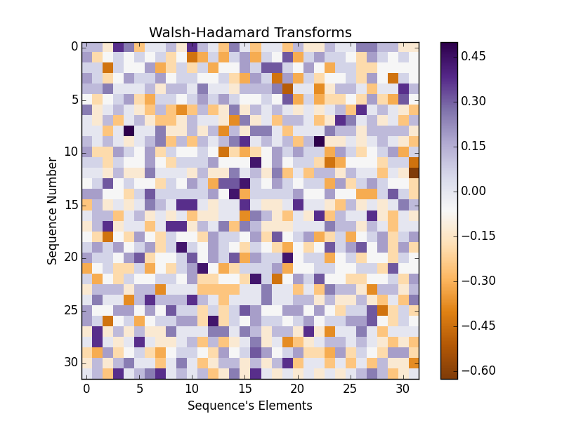
Again, every element (a square) in the above figure corresponds to $w_{ij}$ value. I would like also pay your attention to the fact that both arrays of $t$ and $P$ are 1D vectors storing all t-statistics and $p$-values, respectively. In the following WHT tests we will make an additional effort to split them into $a\times b$ matrices corresponding exactly to $w$-like arrangement. That’s an easy part so don’t bother too much about that.

2.3. Statistical Test Framework

In general, here, we are interested in verification of two opposite statistical hypotheses. The concept of hypothesis testing is given in every textbook on the subject. We test our binary signal $x(t)$ for randomness. Therefore, $H_0$: $x(t)$ is generated by a binary memory-less source i.e. the signal does not contain any predictable component; $H_1$: $x(t)$ is not produced by a binary memory-less source, i.e. the signal contains a predictable component.

Within the standard framework of hypothesis testing we can make two errors. The first one refers to $\alpha$ (so-called significance level) and denotes the probability of occurrence of a false positive result. The second one refers to $\beta$ and denotes the probability of the occurrence of a false negative result.

The testing procedure that can be applied here is: for a fixed value of $\alpha$ we find a confidence region for the test statistic and check if the statistical test value is in the confidence region. The confidence levels are computed using the quantiles $u_{\alpha/2}$ and $u_{1-\alpha/2}$ (otherwise, specified in the text of the test). Alternatively, if an arbitrary $t_{\rm stat}$ is the value of the test statistics (test function) we may compare $p{\rm-value}={\rm Pr}(X\lt t_{\rm stat})$ with $\alpha$ and decide on randomness when $p$-value$\ \ge\alpha$.

2.4. Crude Decision (Test 1)

The first WHT test from the Op09’s suite is a crude decision or majority decision. For chosen $\alpha$ and at $u_\alpha$ denoting the quantile of order $\alpha$ of the normal distribution, if:
$$
t_{ij} \notin [u_{\alpha/2}; u_{1-\alpha/2}] $$ then reject the hypothesis of randomness regarding $i$-th test statistic of the signal $x(t)$ at the significance level of $\alpha$. Jot down both $j$ and $i$ corresponding to sequence number and sequence’s element, respectively. Op09 suggest that this test is suitable for small numbers of $a<1/\alpha\ $ which is generally always fulfilled for our data. We code this test in Python as follows: [code lang="python" gutter="false"] def test1(cl,t,a,b,otest): alpha=1.-cl/100. u1=norm.ppf(alpha/2.) u2=norm.ppf(1-alpha/2.) Results1=[] for l in t: if(l<u1 or l>u2): Results1.append(0) else: Results1.append(1) nfail=a*b-np.sum(Results1) print("Test 1 (Crude Decision)") print(" RESULT: %d out of %d test variables stand for " \ "randomness" % (a*b-nfail,a*b)) if((a*b-nfail)/float(a*b)>.99): print("\t Signal x(t) appears to be random") else: print("\t Signal x(t) appears to be non-random") otest.append(100.*(a*b-nfail)/float(a*b)) # gather per cent of positive results print("\t at %.5f%% confidence level" % (100.*(1.-alpha))) print return(otest) [/code] Op09's decision on rejection of $H_0$ is too stiff. In the function we calculate the number of $t_{ij}$'s falling outside the test interval. If their number exceeds 1%, we claim on the lack of evidence of randomness for $x(t)$ as a whole. 2.5. Proportion of Sequences Passing a Test (Test 2)

Recall that for each row (sub-sequence of $x(t)$) and its elements, we have computed both $t_{ij}$’s and $P_{ij}$ values. Let’s use the latter here. In this test, first, we check for every row of (re-shaped) $t$ 2D array a number of $p$-values to be $P_{ij}\lt\alpha$. If this number is greater than zero, we reject $j$-th sub-sequence of $x(t)$ at the significance level of $\alpha$ to pass the test. For all $a$ sub-sequences we count its total number of those which did not pass the test, $n_2$. If:
$$
n_2 \notin \left[ a\alpha \sqrt{a \alpha (1-\alpha))} u_{\alpha/2}; a\alpha \sqrt{a \alpha (1-\alpha))} u_{1-\alpha/2} \right] $$ then there is evidence that signal $x(t)$ is non-random.

We code this test simply as:

def test2(cl,P,a,b,otest):
    alpha=1.-cl/100.
    u1=norm.ppf(alpha/2.)
    u2=norm.ppf(1-alpha/2.)
    Results2=[]
    rP=np.reshape(P,(a,b))  # turning P 1D-vector into (a x b) 2D array!
    for j in xrange(a):
        tmp=rP[j][(rP[j]<alpha)]
        #print(tmp)
        if(len(tmp)>0):
            Results2.append(0)   # fail for sub-sequence
        else:
            Results2.append(1)   # pass

    nfail2=a-np.sum(Results2)  # total number of sub-sequences which failed
    t2=nfail2/float(a)
    print("Test 2 (Proportion of Sequences Passing a Test)")
    b1=alpha*a+sqrt(a*alpha*(1-alpha))*u1
    b2=alpha*a+sqrt(a*alpha*(1-alpha))*u2
    if(t2<b1 or t2>b2):
        print("  RESULT: Signal x(t) appears to be non-random")
        otest.append(0.)
    else:
        print("  RESULT: Signal x(t) appears to be random")
        otest.append(100.)
    print("\t  at %.5f%% confidence level" % (100.*(1.-alpha)))
    print
    return(otest)

This test is also described well by Rukhin et al. (2010) though we follow the method of Op09 adjusted for the proportion of $p$-values failing the test for randomness as counted sub-sequence by sub-sequence.

2.7. Uniformity of p-values (Test 3)

In this test, the distribution of $p$-values is examined to ensure uniformity. This may be visually illustrated using a histogram, whereby, the interval between 0 and 1 is divided into $K=10$ sub-intervals, and the $p$-values, i.e. in our case $P_{ij}$’s, that lie within each sub-interval are counted and displayed.

Uniformity may also be determined via an application of a $\chi^2$ test and the determination of a $p$-value corresponding to the Goodness-of-Fit Distributional Test on the $p$-values obtained for an arbitrary statistical test (i.e., a $p$-value of the $p$-values). We accomplish that via computation of the test statistic:
$$
\chi^2 = \sum_{i=1}^{K} \frac{\left( F_i-\frac{a}{K} \right)^2}{\frac{a}{K}}
$$ where $F_i$ is the number of $P_{ij}$ in the histogram’s bin of $i$, and $a$ is the number of sub-sequences of $x(t)$ we investigate.

We reject the hypothesis of randomness regarding $i$-th test statistic $t_{ij}$ of $x(t)$ at the significance level of $\alpha$ if:
$$
\chi^2_i \notin [0; \chi^2(\alpha, K-1)] \ .
$$ Let $\chi^2(\alpha, K-1)$ be the quantile of order $\alpha$ of the distribution $\chi^2(K-1)$. In Python we may calculated it in the following way:

from scipy.stats import chi2
alpha=0.001
K=10
# for some derived variable of chi2_test
print(Chi2(alpha,K-1))

If our test value of Test 3 $\chi_i^2\le \chi^2(\alpha, K-1)$ then we count $i$-th statistics to be not against randomness of $x(t)$. This is an equivalent to testing $i$-th $p$-value of $P_{ij}$ if $P_{ij}\ge\alpha$. The latter can be computed in Python as:

from scipy.special import gammainc
alpha=0.001
K=10
# for some derived variable of chi2_test
pvalue=1-gammainc((K-1)/2.,chi2_test/2.)

where gammainc(a,x) stands for incomplete gamma function defined as:
$$
\Gamma(a,x) = \frac{1}{\Gamma(a)} \int_0^x e^{-t} t^{a-1} dt
$$ and $\Gamma(a)$ denotes a standard gamma function.

Given that, we code Test 3 of Uniformity of $p$-values in the following way:

def test3(cl,P,a,b,otest):
    alpha=1.-cl/100.
    rP=np.reshape(P,(a,b))
    rPT=rP.T
    Results3=0
    for i in xrange(b):
        (hist,bin_edges,_)=plt.hist(rPT[i], bins=list(np.arange(0.0,1.1,0.1)))
        F=hist
        K=len(hist)  # K=10 for bins as defined above
        S=a
        chi2=0
        for j in xrange(K):
            chi2+=((F[j]-S/K)**2.)/(S/K)
        pvalue=1-gammainc(9/2.,chi2/2.)
        if(pvalue>=alpha and chi2<=Chi2(alpha,K-1)):
            Results3+=1
    print("Test 3 (Uniformity of p-values)")
    print("  RESULT: %d out of %d test variables stand for randomness"\
          % (Results3,b))
    if((Results3/float(b))>.99):
        print("\t  Signal x(t) appears to be random")
    else:
        print("\t  Signal x(t) appears to be non-random")
    otest.append(100.*(Results3/float(b)))
    print("\t  at %.5f%% confidence level" % (100.*(1.-alpha)))
    print
    return(otest)

where again we allow for less than 1% of all results not to stand against the rejection of $x(t)$ as random signal.

Please note on the transposition of rP matrix. The reason for testing WHT’s values (converted to $t_{ij}$’s or $P_{ij}$’s) is to detect autocorrelation patterns in the tested signal $x(t)$. The same approach has been applied by Op09 in Test 4 and Test 5 as discussed in the following sections and constitutes the core of invention and creativity added to Rukhin et al. (2010)’s suite of 16 tests for signals generated by various PRNGs to meet the cryptographic levels of acceptance as close-to-truly random.

2.8. Maximum Value Decision (Test 4)

This test is based again on the confidence levels approach. Let $T_{ij}=\max_j t_{ij}$ then if:
$$
T_{ij} \notin \left[ u_{\left(\frac{\alpha}{2}\right)^{a^{-1}}}; u_{\left(1-\frac{\alpha}{2}\right)^{a^{-1}}} \right] $$ then reject the hypothesis of randomness (regarding $i$-th test function) of signal $x(t)$ at the significance level of $\alpha$. We encode it to Python no simpler as that:

def test4(cl,t,a,b,otest):
    alpha=1.-cl/100.
    rt=np.reshape(t,(a,b))
    rtT=rt.T
    Results4=0
    for i in xrange(b):
        tmp=np.max(rtT[i])
        u1=norm.ppf((alpha/2.)**(1./a))
        u2=norm.ppf((1.-alpha/2.)**(1./a))
        if not(tmp<u1 or tmp>u2):
            Results4+=1
    print("Test 4 (Maximum Value Decision)")
    print("  RESULT: %d out of %d test variables stand for randomness" % (Results4,b))
    if((Results4/float(b))>.99):
        print("\t  Signal x(t) appears to be random")
    else:
        print("\t  Signal x(t) appears to be non-random")
    otest.append(100.*(Results4/float(b)))
    print("\t  at %.5f%% confidence level" % (100.*(1.-alpha)))
    print
    return(otest)

Pay attention how this test looks at the results derived based on WHTs. It is sensitive to the distribution of maximal values along $i$-th’s elements of $t$-statistics.

2.9. Sum of Square Decision (Test 5)

Final test makes use of the $C$-statistic designed as:
$$
C_i = \sum_{j=0}^{a-1} t_{ij}^2 \ .
$$ If $C_i \notin [0; \chi^2(\alpha, a)]$ we reject the hypothesis of randomness of $x(t)$ at the significance level of $\alpha$ regarding $i$-th test function. The Python reflection of this test finds its form:

def test5(cl,t,a,b,otest):
    alpha=1.-cl/100.
    rt=np.reshape(t,(a,b))
    rtT=rt.T
    Results5=0
    for i in xrange(b):
        Ci=0
        for j in xrange(a):
           Ci+=(rtT[i][j])**2.
        if(Ci<=Chi2(alpha,a)):
            Results5+=1
    print("Test 5 (Sum of Square Decision)")
    print("  RESULT: %d out of %d test variables stand for randomness" % (Results5,b))
    if((Results5/float(b))>.99):
        print("\t  Signal x(t) appears to be random")
    else:
        print("\t  Signal x(t) appears to be non-random")
    otest.append(100.*(Results5/float(b)))
    print("\t  at %.5f%% confidence level" % (100.*(1.-alpha)))
    print
    return(otest)

Again, we allow of 1% of false negative results.

2.10. The Overall Test for Randomness of Binary Signal

We accept signal $x(t)$ to be random if the average passing rate from all five WHT statistical tests is greater than 99%, i.e. 1% can be due to false negative results, at the significance level of $\alpha$.

def overalltest(cl,otest):
    alpha=1.-cl/100.
    line()
    print("THE OVERALL RESULT:")
    if(np.mean(otest)>=99.0):
        print("   Signal x(t) displays an evidence for RANDOMNESS"),
        T=1
    else:
        print("   Signal x(t) displays an evidence for NON-RANDOMNESS"),
        T=0
    print("at %.5f%% c.l." % (100.*(1.-alpha)))
    print("   based on Walsh-Hadamard Transform Statistical Test\n")
    return(T)

and run all 5 test by calling the following function:

def WHTStatTest(cl,X):
    (xseq,xt,a,b,M) = xsequences(X)
    info(X,xt,a,b,M)
    if(M<7):
        line()
        print("Error:  Signal x(t) too short for WHT Statistical Test")
        print("        Acceptable minimal signal length: n=2^7=128\n")
    else:
        if(M>=7 and M<19):
            line()
            print("Warning: Statistically advisable signal length: n=2^19=524288\n")
        line()
        print("Test Name: Walsh-Hadamard Transform Statistical Test\n")
        (t, P, _) = tstat(xseq,a,b,M)
        otest=test1(cl,t,a,b,[])
        otest=test2(cl,P,a,b,otest)
        otest=test3(cl,P,a,b,otest)
        otest=test4(cl,t,a,b,otest)
        otest=test5(cl,t,a,b,otest)
        T=overalltest(cl,otest)
        return(T)  # 1 if x(t) is random

fed by binary $\pm 1$ signal of $X$ (see example in Section 2.1). The last function return T variable storing $1$ for the overall decision that $x(t)$ is random, $0$ otherwise. It can be used for a great number of repeated WHT tests for different signals in a loop, thus for determination of ratio of instances the WHT Statistical Test passed.

3. Randomness of random()

I know what you think right now. I have just spent an hour reading all that stuff so far, how about some real-life tests? I’m glad you asked! Here we go! We start with Mersenne Twister algorithm being the Rolls-Royce engine of Python’s random() function (and its derivatives). The whole fun of the theoretical part given above comes down to a few lines of code as given below.

Let’s see our WHT Suite of 5 Statistical Tests in action for a very long (of length $n=2^{21}$) random binary signal of $\pm 1$ form. Let’s run the exemplary main program calling the test:

# Walsh-Hadamard Transform and Tests for Randomness of Financial Return-Series
# (c) 2015 QuantAtRisk.com, by Pawel Lachowicz
#
# Mersenne Twister PRNG test using WHT Statistical Test

from WalshHadamard import WHTStatTest, line
from random import randrange

# define confidence level for WHT Statistical Test
cl=99.9999

# generate random binary signal X(t)
X=[randrange(-1,2,2) for i in xrange(2**21)]
line()
print("X(t) =")
for i in range(20):
    print(X[i]),
print("...")

WHTStatTest(cl,X)

what returns lovely results, for instance:

----------------------------------------------------------------------
X(t) =
-1 -1 1 1 1 -1 1 -1 1 1 1 1 1 -1 -1 1 1 -1 1 1 ...
----------------------------------------------------------------------
Signal		X(t)
  of length	n = 2097152 digits
trimmed to	x(t)
  of length	n = 2097152 digits (n=2^21)
  split into	a = 1024 sub-sequences 
		b = 2048-digit long

----------------------------------------------------------------------
Test Name: Walsh-Hadamard Transform Statistical Test

Computation of WHTs...
  ...completed
Computation of t-statistics... completed
Computation of p-values... completed

Test 1 (Crude Decision)
  RESULT: 2097149 out of 2097152 test variables stand for randomness
	  Signal x(t) appears to be random
	  at 99.99990% confidence level

Test 2 (Proportion of Sequences Passing a Test)
  RESULT: Signal x(t) appears to be random
	  at 99.99990% confidence level

Test 3 (Uniformity of p-values)
  RESULT: 2045 out of 2048 test variables stand for randomness
	  Signal x(t) appears to be random
	  at 99.99990% confidence level

Test 4 (Maximum Value Decision)
  RESULT: 2047 out of 2048 test variables stand for randomness
	  Signal x(t) appears to be random
	  at 99.99990% confidence level

Test 5 (Sum of Square Decision)
  RESULT: 2048 out of 2048 test variables stand for randomness
	  Signal x(t) appears to be random
	  at 99.99990% confidence level

----------------------------------------------------------------------
THE OVERALL RESULT:
   Signal x(t) displays an evidence for RANDOMNESS at 99.99990% c.l.
   based on Walsh-Hadamard Transform Statistical Test

where we assumed the significance level of $\alpha=0.000001$. Impressive indeed!

A the same $\alpha$ however for shorter signal sub-sequencies ($a=256; n=2^{16}$), we still get a significant number of passed tests supporting randomness of random(), for instance:

----------------------------------------------------------------------
X(t) =
-1 -1 1 -1 1 1 1 1 1 -1 -1 -1 -1 -1 -1 1 1 -1 1 -1 ...
----------------------------------------------------------------------
Signal		X(t)
  of length	n = 65536 digits
trimmed to	x(t)
  of length	n = 65536 digits (n=2^16)
  split into	a = 256 sub-sequences 
		b = 256-digit long

----------------------------------------------------------------------
Warning: Statistically advisable signal length: n=2^19=524288

----------------------------------------------------------------------
Test Name: Walsh-Hadamard Transform Statistical Test

Computation of WHTs...
  ...completed
Computation of t-statistics... completed
Computation of p-values... completed

Test 1 (Crude Decision)
  RESULT: 65536 out of 65536 test variables stand for randomness
	  Signal x(t) appears to be random
	  at 99.99990% confidence level

Test 2 (Proportion of Sequences Passing a Test)
  RESULT: Signal x(t) appears to be random
	  at 99.99990% confidence level

Test 3 (Uniformity of p-values)
  RESULT: 254 out of 256 test variables stand for randomness
	  Signal x(t) appears to be random
	  at 99.99990% confidence level

Test 4 (Maximum Value Decision)
  RESULT: 255 out of 256 test variables stand for randomness
	  Signal x(t) appears to be random
	  at 99.99990% confidence level

Test 5 (Sum of Square Decision)
  RESULT: 256 out of 256 test variables stand for randomness
	  Signal x(t) appears to be random
	  at 99.99990% confidence level

----------------------------------------------------------------------
THE OVERALL RESULT:
   Signal x(t) displays an evidence for RANDOMNESS at 99.99990% c.l.
   based on Walsh-Hadamard Transform Statistical Test

For this random binary signal $x(t)$, the Walsh-Hadamard Transforms for the first 64 signal sub-sequences reveal pretty “random” distributions of $w_{ij}$ values:

4. Randomness of Financial Return-Series

Eventually, we stand face to face in the grand finale with the question: do financial return time-series can be of random nature? More precisely, if we convert any return-series (regardless of time step, frequency of trading, etc.) to the binary $\pm 1$ signal, do the corresponding positive and negative returns occur randomly or not? Good question.

Let’s see by example of FX 30-min return-series of USDCHF currency pair traded between Sep/2009 and Nov/2014, how our WHT test for randomness works. We use the tick-data downloaded from Pepperstone.com and rebinned up to 30-min evenly distributed price series as provided in my earlier post of Rebinning Tick-Data for FX Algo Traders. We read the data by Python and convert the price-series into return-series.

What follows is similar what we have done within previous examples. First, we convert the return-series into binary signal. As we will see, the signal $X(t)$ is 65732 point long and can be split into 256 sub-sequences 256-point long. Therefore $n=2^{16}$ stands for the trimmed signal of $x(t)$. For the same of clarity, we plot first 64 segments (256-point long) for the USDCHF price-series marking all segments with vertical lines. Next, we run the WHT Statistical Test for all $a=256$ sequences but we display WHTs for only first 64 blocks as visualised for the price-series. The main code takes form:

# Walsh-Hadamard Transform and Tests for Randomness of Financial Return-Series
# (c) 2015 QuantAtRisk.com, by Pawel Lachowicz
#
# 30-min FX time-series (USDCHF) traded between 9/2009 and 11/2014

from WalshHadamard import WHTStatTest, ret2bin, line as Line
import matplotlib.pyplot as plt
import numpy as np
import csv

# define confidence level for WHT Statistical Test
cl=99.9999

# open the file and read in the 30min price of USD/CHF
P=[]
with open("USDCHF.30m") as f:
    c = csv.reader(f, delimiter=' ', skipinitialspace=True)
    for line in c:
        price=line[6]
        P.append(price)

x=np.array(P,dtype=np.float128) # convert to numpy array
r=x[1:]/x[0:-1]-1.  # get a return-series
Line()
print("r(t) =")
for i in range(7):
    print("%8.5f" % r[i]),
print("...")

X=ret2bin(r)
print("X(t) =")
for i in range(7):
    print("%8.0f" %X[i]),
print("...")

plt.plot(P)
plt.xlabel("Time (from 1/05/2009 to 27/09/2010)")
plt.ylabel("USDCHF (30min)")
#plt.xlim(0,len(P))
plt.ylim(0.95,1.2)
plt.xlim(0,64*256)
plt.gca().xaxis.set_major_locator(plt.NullLocator())
for x in range(0,256*265,256):
    plt.hold(True)
    plt.plot((x,x), (0,10), 'k-')
plt.show()
plt.close("all")

WHTStatTest(cl,X)

and displays both plots as follows: (a) USDCHF clipped price-series,

and (b) WFTs for first 64 sequences 256-point long,

From the comparison of both figures one can understand the level of details how WHT results are derived. Interesting, for FX return-series, the WHT picture seems to be quite non-uniform suggesting that our USDCHF return-series is random. Is it so? The final answer deliver the results of WHT statistical test, summarised by our program as follows:

----------------------------------------------------------------------
r(t) =
-0.00092 -0.00033 -0.00018  0.00069 -0.00009 -0.00003 -0.00086 ...
X(t) =
      -1       -1       -1        1       -1       -1       -1 ...
----------------------------------------------------------------------
Signal		X(t)
  of length	n = 65731 digits
trimmed to	x(t)
  of length	n = 65536 digits (n=2^16)
  split into	a = 256 sub-sequences 
		b = 256-digit long

----------------------------------------------------------------------
Warning: Statistically advisable signal length: n=2^19=524288

----------------------------------------------------------------------
Test Name: Walsh-Hadamard Transform Statistical Test

Computation of WHTs...
  ...completed
Computation of t-statistics... completed
Computation of p-values... completed

Test 1 (Crude Decision)
  RESULT: 65536 out of 65536 test variables stand for randomness
	  Signal x(t) appears to be random
	  at 99.99990% confidence level

Test 2 (Proportion of Sequences Passing a Test)
  RESULT: Signal x(t) appears to be random
	  at 99.99990% confidence level

Test 3 (Uniformity of p-values)
  RESULT: 250 out of 256 test variables stand for randomness
	  Signal x(t) appears to be non-random
	  at 99.99990% confidence level

Test 4 (Maximum Value Decision)
  RESULT: 255 out of 256 test variables stand for randomness
	  Signal x(t) appears to be random
	  at 99.99990% confidence level

Test 5 (Sum of Square Decision)
  RESULT: 256 out of 256 test variables stand for randomness
	  Signal x(t) appears to be random
	  at 99.99990% confidence level

----------------------------------------------------------------------
THE OVERALL RESULT:
   Signal x(t) displays an evidence for RANDOMNESS at 99.99990% c.l.
   based on Walsh-Hadamard Transform Statistical Test

Nice!! Wasn’t worth it all the efforts to see this result?!

I’ll leave you with a pure joy of using the software I created. There is a lot to say and a lot to verify. Even the code itself can be amended a bit and adjusted for different sequence number $a$ and $b$’s. If you discover a strong evidence for non-randomness, post it in comments or drop me an e-mail. I can’t do your homework. It’s your turn. I need to sleep sometimes… ;-)

DOWNLOAD
     WalshHadamard.py, USDCHF.30m