Conversion of Financial Time Series based on Daily Returns Matrix in Python

As a financial analyst or algo trader, you are so often faced with information on, inter alia, daily asset trading in a form of a daily returns matrix. In many cases, it is easier to operate with the return-series rather than with price-series. And there are excellent reasons standing behind such decision, e.g. the possibility to plot the histogram of daily returns, the calculation of daily Value-at-Risk (Var), etc.

When you use Python (not Matlab), the recovery of price-series for return-series may be a bit of challenge, especially when you face the problem for the first time. A technical problem, i.e. “how to do it?!” within Python, requires you to switch your thinking mode and adjust your vantage point from Matlab-ish to Pythonic. Therefore, let’s see what is the best recipe to turn your world upside down?!

Say, we start with a $N$-asset portfolio of $N$ assets traded for $L+1$ last days. It will require the use of the Python’s NumPy arrays. We begin with:

import numpy as np
import matplotlib.pyplot as plt

np.random.seed(2014)

# define portfolio
N = 5  # number of assets
L = 4  # number of days

# asset close prices
p = np.random.randint(10, 30, size=(N, 1)) + \
    np.random.randn(N, 1)  # a mixture of uniform and N(0,1) rvs
print(p)
print(p.shape)
print()

where we specify a number of assets in portfolio and a number of days. $L = 4$ has been selected for the clarity of printing of the outcomes below, however, feel free to increase that number (or both) anytime you rerun this code.

Next, we create a matrix ($N\times 1$) with a starting random prices for all $N$ assets to be between \$10 and \$30 (random integer) supplemented by (0, 1) fractional part. Printing p returns:

[[ 25.86301396]
 [ 19.82072772]
 [ 22.33569347]
 [ 21.38584671]
 [ 24.56983489]]
(5, 1)

Now, let’s generate a matrix of random daily returns over next 4 days for all 5 assets:

r = np.random.randn(N, L)/50
print(r)
print(r.shape)

delivering:

[[ 0.01680965 -0.00620443 -0.02876535 -0.03946471]
 [-0.00467748 -0.0013034   0.02112921  0.01095789]
 [-0.01868982 -0.01764086  0.01275301  0.00858922]
 [ 0.01287237 -0.00137129 -0.0135271   0.0080953 ]
 [-0.00615219 -0.03538243  0.01031361  0.00642684]]
(5, 4)

Having that, our wish is, for each asset, take its first close-price value from the p array and using information on daily returns stored row-by-row (i.e. asset per asset) in the r array, reconstruct the close-price asset time-series:

for i in range(r.shape[0]):
    tmp = []
    for j in range(r.shape[1]):
        if(j == 0):
            tmp.append(p[i][0].tolist())
            y = p[i] * (1 + r[i][j])
        else:
            y = y * (1 + r[i][j])
        tmp.append(y.tolist()[0])

    if(i == 0):
        P = np.array(tmp)
    else:
        P = np.vstack([P, np.array(tmp)])

print()
print(P)
print(P.shape)
print()

That returns:

[[ 25.86301396  26.29776209  26.13459959  25.38282873  24.38110263]
 [ 19.82072772  19.72801677  19.70230331  20.11859739  20.33905475]
 [ 22.33569347  21.91824338  21.53158666  21.8061791   21.99347727]
 [ 21.38584671  21.66113324  21.63142965  21.33881915  21.51156325]
 [ 24.56983489  24.41867671  23.55468454  23.79761839  23.95056194]]
(5, 5)

Thus, we have two loops: the outer one over rows/assets (index i) and inner one over columns/days (index j). For j = 0 we copy the price of the asset from p as a “starting close price”, e.g. on the first day. Concurrently, using the first information from r matrix we compute a change in price on the next day. In tmp list we store (per asset) the history of close price changes over all L+1 days. These operations are based on a simple list processing. Finally, having a complete information on i-th asset and its price changes after r.shape[1] + 1 days, we build a new array of P with an aid of np.vstack function (see more in Section 3.3.4 of Python for Quants. Volume I). Therefore, P stores the simulated close-price time-series for N assets.

We can display them by adding to our main code:

plt.figure(num=1, figsize=(8, 5))
plt.plot(P.T, '+-')
plt.xlabel("Days")
plt.ylabel("Asset Close Price (\$)")

what reveals:

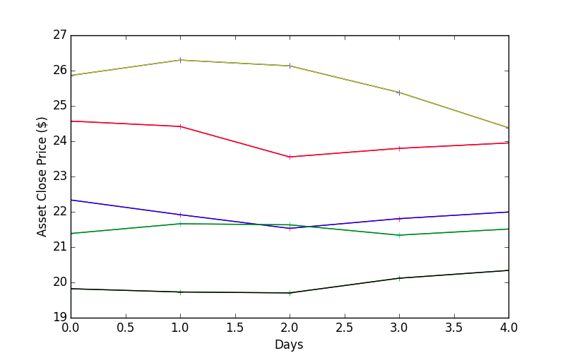
where the transposition of P for plotting has been applied to deliver asset-by-asset price-series (try to plot the array without it and see what happens and understand why it is so).

The easiest solutions are most romantic, what we have proven above. You don’t impress your girlfriend by buying 44 red roses. 44 lines of Python code will do the same! Trust me on that! ;-)

This lesson comes from a fragment of my newest book of Python for Quants. Volume I. The bestselling book in a timeframe of last 3 days after publishing!