Student t Distributed Linear Value-at-Risk

One of the most underestimated feature of the financial asset distributions is their kurtosis. A rough approximation of the asset return distribution by the Normal distribution becomes often an evident exaggeration or misinterpretations of the facts. And we know that. The problem arises if we investigate a linear Value-at-Risk (VaR) measure. Within a standard approach, it is computed based on the analytical formula:
$$
\mbox{VaR}_{h, \alpha} = \Phi ^{-1} (1-\alpha)\sqrt{h}\sigma – h\mu
$$ what expresses $(1-\alpha)$ $h$-day VaR, $\Phi ^{-1} (1-\alpha)$ denotes the standardised Normal distribution $(1-\alpha)$ quantile, and $h$ is a time horizon. The majority of stocks display significant excess kurtosis and negative skewness. In plain English that means that the distribution is peaked and likely to have a heavy left tail. In this scenario, the best fit of the Normal probability density function (pdf) to the asset return distribution underestimates the risk accumulated in a far negative territory.

In this post we will introduce the concept of Student t Distributed Linear VaR, i.e. an alternative method to measure VaR by taking into account “a correction” for kurtosis of the asset return distribution. We will use the market stock data of IBM as an exemplary case study and investigate the difference in a standard and non-standard VaR calculation based on the parametric models. It will also be an excellent opportunity to learn how to do it in Python, quickly and effectively.

1. Leptokurtic Distributions and Linear Value-at-Risk

A leptokurtic distribution is one whose density function has a higher peak and greater mass in the tails than the normal density function of the same variance. In a symmetric unimodal distribution, i.e. one whose density function has only one peak, leptokurtosis is indicated by a positive excess kurtosis (Alexander 2008). The impact of leptokurtosis on VaR is non-negligible. Firstly, assuming high significance levels, e.g. $\alpha \le 0.01$, the estimation of VaR for Normal and leptokurtic distribution would return:
$$
\mbox{VaR}_{lepto,\ \alpha\le 0.01} \gt \mbox{VaR}_{Norm,\ \alpha\le 0.01}
$$
which is fine, however for low significance levels the situation may change:
$$
\mbox{VaR}_{lepto,\ \alpha\ge 0.05} \lt \mbox{VaR}_{Norm,\ \alpha\ge 0.05} \ .
$$
A good example of the leptokurtic distribution is Student t distribution. If it describes the data better and displays significant excess kurtosis, there is a good chance that VaR for high significance levels will be a much better measure of the tail risk. The Student t distribution is formally given by its pdf:
$$
f_\nu(x) = \sqrt{\nu\pi} \Gamma\left(\frac{\nu}{2}\right)^{-1} \Gamma\left(\frac{\nu+1}{2}\right)
(1+\nu^{-1} x^2)^{-(\nu+1)/2}
$$ where $\Gamma$ denotes the gamma function and $\nu$ the degrees of freedom. For $\nu\gt 2$ its variance is $\nu(\nu-2)^{-1}$ and the distribution has a finite excess kurtosis of $\kappa = 6(\nu-4)^{-1}$ for $\nu \gt 4$. It is obvious that for $\nu\to \infty$ the Student t pdf approaches the Normal pdf. Large values of $\nu$ for the fitted Student t pdf in case of the financial asset daily return distribution are unlikely, unless the Normal distribution is the best pdf model indeed (possible to obtain for very large samples).

We find $\alpha$ quantile of the Student t distribution ($\mu=0$ and $\sigma=1$) by the integration of the pdf and usually denote it as $\sqrt{\nu^{-1}(\nu-2)} t_{\nu}^{-1}(\alpha)$ where $t_{\nu}^{-1}$ is the percent point function of the t distribution. Accounting for the fact that in practice we deal with random variables of the form of $X = \mu + \sigma T$ where $X$ would describe the asset return given as a transformation of the standardised Student t random variable, we reach to the formal definition of the $(1-\alpha)$ $h$-day Student t VaR given by:
$$
\mbox{Student}\ t\ \mbox{VaR}_{\nu, \alpha, h} = \sqrt{\nu^{-1}(\nu-2)h}\ t_{\nu}^{-1}(1-\alpha)\sigma – h\mu
$$ Having that, we are ready to use this knowledge in practice and to understand, based on data analysis, the best regimes where one should (and should not) apply the Student t VaR as a more “correct” measure of risk.

2. Normal and Student t VaR for IBM Daily Returns

Within the following case study we will make of use of Yahoo! Finance data provider in order to fetch the price-series of the IBM stock (adjusted close) and transform it into return-series. As the first task we have to verify before heading further down this road will be the sample skewness and kurtosis. We begin, as usual:

# Student t Distributed Linear Value-at-Risk
#   The case study of VaR at the high significance levels
# (c) 2015 Pawel Lachowicz, QuantAtRisk.com

import numpy as np
import math
from scipy.stats import skew, kurtosis, kurtosistest
import matplotlib.pyplot as plt
from scipy.stats import norm, t
import pandas_datareader.data as web


# Fetching Yahoo! Finance for IBM stock data
data = web.DataReader("IBM", data_source='yahoo',
                  start='2010-12-01', end='2015-12-01')['Adj Close']
cp = np.array(data.values)  # daily adj-close prices
ret = cp[1:]/cp[:-1] - 1    # compute daily returns

# Plotting IBM price- and return-series
plt.figure(num=2, figsize=(9, 6))
plt.subplot(2, 1, 1)
plt.plot(cp)
plt.axis("tight")
plt.ylabel("IBM Adj Close [USD]")
plt.subplot(2, 1, 2)
plt.plot(ret, color=(.6, .6, .6))
plt.axis("tight")
plt.ylabel("Daily Returns")
plt.xlabel("Time Period 2010-12-01 to 2015-12-01 [days]")

where we cover the most recent past 5 years of trading of IBM at NASDAQ. Both series visualised look like:

where, in particular, the bottom one reveals five days where the stock experienced 5% or higher daily loss.

In Python, a correct computation of the sample skewness and kurtosis is possible thanks to the scipy.stats module. As a test you may verify that for a huge sample (e.g. of 10 million) of random variables $X\sim N(0, 1)$, the expected skewness and kurtosis,

from scipy.stats import skew, kurtosis
X = np.random.randn(10000000)
print(skew(X))
print(kurtosis(X, fisher=False))

is indeed equal 0 and 3,

0.0003890933008049
3.0010747070253507

respectively.

As we will convince ourselves in a second, this is not the case for our IBM return sample. Continuing,

print("Skewness  = %.2f" % skew(ret))
print("Kurtosis  = %.2f" % kurtosis(ret, fisher=False))
# H_0: the null hypothesis that the kurtosis of the population from which the
# sample was drawn is that of the normal distribution kurtosis = 3(n-1)/(n+1)
_, pvalue = kurtosistest(ret)
beta = 0.05
print("p-value   = %.2f" % pvalue)
if(pvalue < beta):
    print("Reject H_0 in favour of H_1 at %.5f level\n" % beta)
else:
    print("Accept H_0 at %.5f level\n" % beta)

we compute the moments and run the (excess) kurtosis significance test. As already explained in the comment, we are interested whether the derived value of kurtosis is significant at $\beta=0.05$ level or not? We find that for IBM, the results reveal:

Skewness  = -0.70
Kurtosis  = 8.39
p-value   = 0.00
Reject H_0 in favour of H_1 at 0.05000 level

id est, we reject the null hypothesis that the kurtosis of the population from which the sample was drawn is that of the normal distribution kurtosis in favour of the alternative hypothesis ($H_1$) that it is not. And if not then we have work to do!

In the next step we fit the IBM daily returns data sample with both Normal pdf and Student t pdf in the following way:

# N(x; mu, sig) best fit (finding: mu, stdev)
mu_norm, sig_norm = norm.fit(ret)
dx = 0.0001  # resolution
x = np.arange(-0.1, 0.1, dx)
pdf = norm.pdf(x, mu_norm, sig_norm)
print("Integral norm.pdf(x; mu_norm, sig_norm) dx = %.2f" % (np.sum(pdf*dx)))
print("Sample mean  = %.5f" % mu_norm)
print("Sample stdev = %.5f" % sig_norm)
print()

# Student t best fit (finding: nu)
parm = t.fit(ret)
nu, mu_t, sig_t = parm
pdf2 = t.pdf(x, nu, mu_t, sig_t)
print("Integral t.pdf(x; mu, sig) dx = %.2f" % (np.sum(pdf2*dx)))
print("nu = %.2f" % nu)
print()

where we ensure that the complete integral over both pdfs return 1, as expected:

Integral norm.pdf(x; mu_norm, sig_norm) dx = 1.00
Sample mean  = 0.00014
Sample stdev = 0.01205

Integral t.pdf(x; mu, sig) dx = 1.00
nu = 3.66

The best fit of the Student t pdf returns the estimate of 3.66 degrees of freedom.

From this point, the last step is the derivation of two distinct VaR measure, the first one corresponding to the best fit of the Normal pdf and the second one to the best fit of the Student t pdf, respectively. The trick is

# Compute VaR
h = 1  # days
alpha = 0.01  # significance level
StudenthVaR = (h*(nu-2)/nu)**0.5 * t.ppf(1-alpha, nu)*sig_norm - h*mu_norm
NormalhVaR = norm.ppf(1-alpha)*sig_norm - mu_norm

lev = 100*(1-alpha)
print("%g%% %g-day Student t VaR = %.2f%%" % (lev, h, StudenthVaR*100))
print("%g%% %g-day Normal VaR    = %.2f%%" % (lev, h, NormalhVaR*100))

that in the calculation of the $(1-\alpha)$ $1$-day Student t VaR ($h=1$) according to:
$$
\mbox{Student}\ t\ \mbox{VaR}_{\nu, \alpha=0.01, h=1} = \sqrt{\nu^{-1}(\nu-2)}\ t_{\nu}^{-1}(0.99)\sigma – \mu
$$ we have to take $\sigma$ and $\mu$ given by sig_norm and mu_norm variable (in the code) and not the ones returned by the t.fit(ret) function in line #54. We find out that:

99% 1-day Student t VaR = 3.19%
99% 1-day Normal VaR    = 2.79%

i.e. VaR derived based on the Normal pdf best fit may underestimate the tail risk for IBM, as suspected in the presence of highly significant excess kurtosis. Since the beauty of the code is aesthetic, the picture is romantic. We visualise the results of our investigation, extending our code with:

plt.figure(num=1, figsize=(11, 6))
grey = .77, .77, .77
# main figure
plt.hist(ret, bins=50, normed=True, color=grey, edgecolor='none')
plt.hold(True)
plt.axis("tight")
plt.plot(x, pdf, 'b', label="Normal PDF fit")
plt.hold(True)
plt.axis("tight")
plt.plot(x, pdf2, 'g', label="Student t PDF fit")
plt.xlim([-0.2, 0.1])
plt.ylim([0, 50])
plt.legend(loc="best")
plt.xlabel("Daily Returns of IBM")
plt.ylabel("Normalised Return Distribution")
# inset
a = plt.axes([.22, .35, .3, .4])
plt.hist(ret, bins=50, normed=True, color=grey, edgecolor='none')
plt.hold(True)
plt.plot(x, pdf, 'b')
plt.hold(True)
plt.plot(x, pdf2, 'g')
plt.hold(True)
# Student VaR line
plt.plot([-StudenthVaR, -StudenthVaR], [0, 3], c='g')
# Normal VaR line
plt.plot([-NormalhVaR, -NormalhVaR], [0, 4], c='b')
plt.text(-NormalhVaR-0.01, 4.1, "Norm VaR", color='b')
plt.text(-StudenthVaR-0.0171, 3.1, "Student t VaR", color='g')
plt.xlim([-0.07, -0.02])
plt.ylim([0, 5])
plt.show() 

what brings us to:

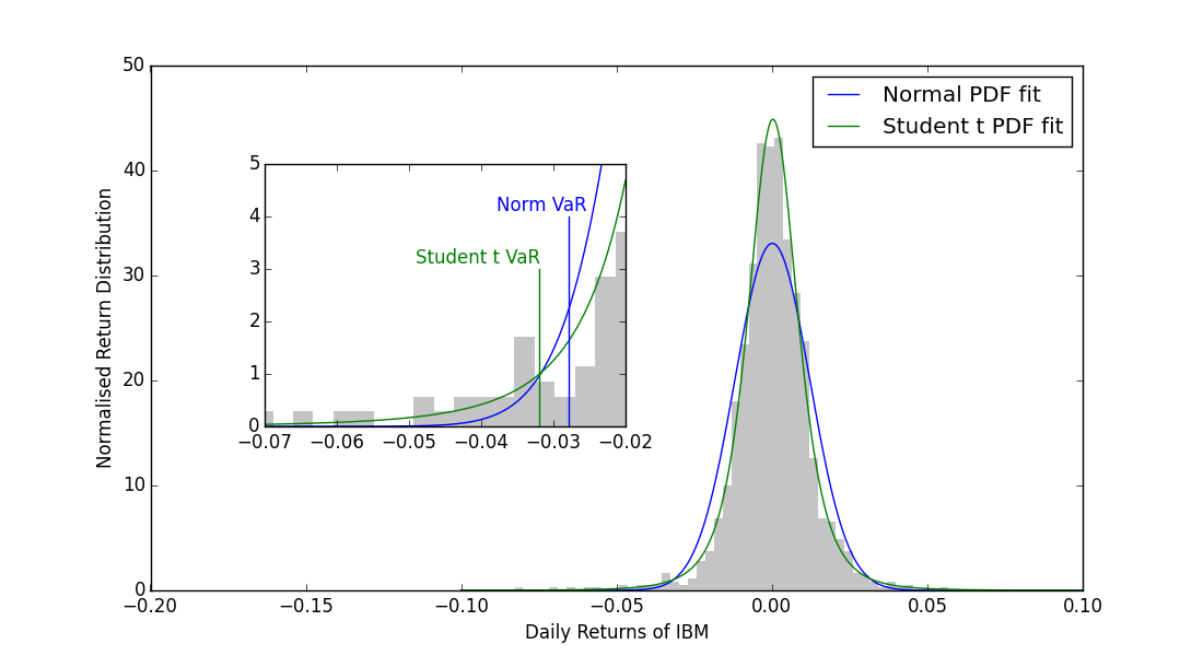
where in the inset, we zoomed in the left tail of the distribution marking both VaR results. Now, it is much clearly visible why at $\alpha=0.01$ the Student t VaR is greater: the effect of leptokurtic distribution. Moreover, the fit of the Student t pdf appears to be a far better parametric model describing the central mass (density) of IBM daily returns.

There is an ongoing debate which one out of these two risk measures should be formally applied when it comes to reporting of 1-day VaR. I do hope that just by presenting the abovementioned results I made you more aware that: (1) it is better to have a closer look at the excess kurtosis for your favourite asset (portfolio) return distribution, and (2) normal is boring.

Someone wise once said: “Don’t be afraid of being different. Be afraid of being the same as everyone else.” The same means normal. Dare to fit non-Normal distributions!

Download

     tStudentVaR.py

References

     Alexander, C., 2008, Market Risk Analysis. Volume IV., John Wiley & Sons Ltd

Explore Further

→ Conditional Value-at-Risk for Normal and Student t Linear VaR Model
→ Student’s t-distribution
→ A VaR assuming Student t distribution not significantly different from a normal VaR