Financial Time Series Segmentation Based On Turning Points in Python

A determination of peaks and troughs for any financial time-series seems to be always in high demand, especially in algorithmic trading. A number of numerical methods can be found in the literature. The main problem exists when a smart differentiation between a local trend and “global” sentiment needs to be translated into computer language. In this short post, we fully refer to the publication of Yin, Si, & Gong (2011) on Financial Time-Series Segmentation using Turning Points wherein the authors proposed an appealing way to simplify the “noisy” character of the financial (high-frequency) time-series.

Since this publication presents an easy-to-digest historical introduction to the problem with a novel pseudo-code addressing solution, let me skip this part here and refer you to the paper itself (download .pdf here).

We develop Python implementation of the pseudo-code as follows. We start with some dataset. Let us use the 4-level order-book record of Hang Seng Index as traded over Jan 4, 2016 (download 20160104_orderbook.csv.zip; 8MB). The data cover both morning and afternoon trading sessions:

import pandas as pd
import numpy as np
import matplotlib.pyplot as plt

# Reading Orderbook
data = pd.read_csv('20160104_orderbook.csv')
data['MidPrice0'] = (data.AskPrice0 + data.BidPrice0)/2.  # mid-price

# Split Data according to Sessions
delta = np.diff(data.Timestamp)
# find a good separation index
k = np.where(delta > np.max(delta)/2)[0][0] + 1

data1 = data[0:k].copy()  # Session 12:15-15:00
data2 = data[k+1:].copy() # Session 16:00-19:15
data2.index = range(len(data2))

plt.figure(figsize=(10,5))
plt.plot(data1.Timestamp, data1.MidPrice0, 'r', label="Session 12:15-15:00")
plt.plot(data2.Timestamp, data2.MidPrice0, 'b', label="Session 16:00-19:15")
plt.legend(loc='best')
plt.axis('tight')

revealing:

Turning Points pseudo-algorithm of Yin, Si, & Gong (2011) can be organised using simple Python functions in a straightforward way, namely:

def first_tps(p):
    tp = []
    for i in range(1, len(p)-1):
        if((p[i] < p[i+1]) and (p[i] < p[i-1])) or ((p[i] > p[i+1]) \
           and (p[i] > p[i-1])):
            tp.append(i)
    return tp

def contains_point_in_uptrend(i, p):
    if(p[i] < p[i+1]) and (p[i] < p[i+2]) and (p[i+1] < p[i+3]) and \
              (p[i+2] < p[i+3]) and \
              (abs(p[i+1] - p[i+2]) < abs(p[i] - p[i+2]) + abs(p[i+1] - p[i+3])):
        return True
    else:
        return False

def contains_point_in_downtrend(i, p):
    if(p[i] > p[i+1]) and (p[i] > p[i+2]) and (p[i+1] > p[i+3]) and \
           (p[i+2] > p[i+3]) and \
           (abs(p[i+2] - p[i+1]) < abs(p[i] - p[i+2]) + abs(p[i+1] - p[i+3])):
        return True
    else:
        return False

def points_in_the_same_trend(i, p, thr):
    if(abs(p[i]/p[i+2]-1) < thr) and (abs(p[i+1]/p[i+3]-1) < thr):
        return True
    else:
        return False

def turning_points(idx, p, thr):
    i = 0
    tp = []
    while(i < len(idx)-3):
        if contains_point_in_downtrend(idx[i], p) or \
           contains_point_in_uptrend(idx[i], p) \
              or points_in_the_same_trend(idx[i], p, thr):
            tp.extend([idx[i], idx[i+3]])
            i += 3
        else:
            tp.append(idx[i])
            i += 1
    return tp

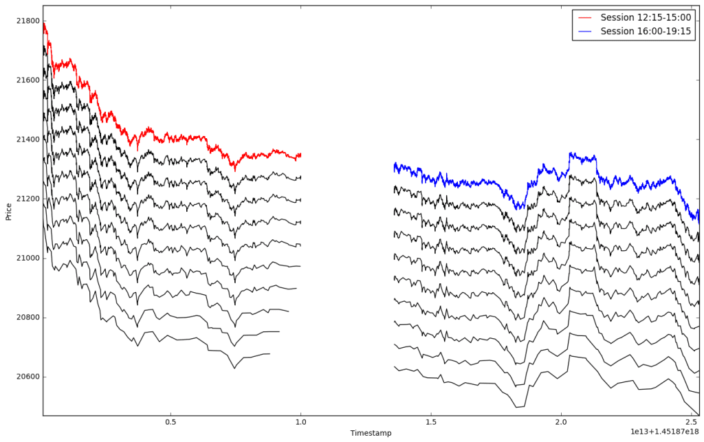
The algorithms allows us to specify a number $k$ (or a range) of sub-levels for time-series segmentation. The “deeper” we go the more distinctive peaks and throughs remain. Have a look:

thr = 0.05
sep = 75  # separation for plotting

P1 = data1.MidPrice0.values
P2 = data2.MidPrice0.values
tp1 = first_tps(P1)
tp2 = first_tps(P2)

plt.figure(figsize=(16,10))

plt.plot(data1.Timestamp, data1.MidPrice0, 'r', label="Session 12:15-15:00")
plt.plot(data2.Timestamp, data2.MidPrice0, 'b', label="Session 16:00-19:15")
plt.legend(loc='best')

for k in range(1, 10):  # k over a given range of sub-levels
    tp1 = turning_points(tp1, P1, thr)
    tp2 = turning_points(tp2, P2, thr)
    plt.plot(data1.Timestamp[tp1], data1.MidPrice0[tp1]-sep*k, 'k')
    plt.plot(data2.Timestamp[tp2], data2.MidPrice0[tp2]-sep*k, 'k')
    
plt.axis('tight')
plt.ylabel('Price')
plt.xlabel('Timestamp')

It is highly tempting to use the code as a supportive indicator for confirmation of new trends in the time-series (single) or build concurrently running decomposition (segmentation; at the same sub-level) for two or more parallel time-series (e.g. of the FX pairs). Enjoy!