When you come in contact with cryptocurrencies, e.g. Bitcoin (BTC), you quickly realise that there is no single price of BTC at any given moment. The reason is that Bitcoin is traded on different markets. It can be worth more on Coinbase exchange and less on Kraken exchange. In particular, the Coindesk Bitcoin Price Index (XBP) aims to unify the BTC price into a single number based on four markets that meet specific criteria (see here for details on XBP calculation). In practice, the use of a cryptocurrency index seems to be valuable for press and newspapers, not for traders and investors. They usually look at the exchange where their positions are opened and track the exchange-related prices.
The idea of trading the same cryptocurrency on different crypto-markets at the same time is not new. It dates back to trading of a pair of stocks (equities) which prices are highly correlated and cointegrated and is known as statistical arbitrage (Stat Arb). The basic statistical arbitrage is a trading strategy that assumes that the price-series of two assets put into a pair (stocks or, in our case, cryptocurrencies) are non-stationary and mean reverting over time. In other words, when one coin in a pair outperforms the other, the poorer performing coin is bought long with the expectation that it will climb towards its outperforming partner, the other is sold short.
In this post we will see how to combine theory with real market data, identify statistical arbitrage opportunities to buy/sell, create a simple backtest in Python to prove that Stat Arb is not dead and, in fact, that you can make money in cryptocurrency markets! Ready for launch? Let’s go!
1. Markets where a given Cryptocurrency is Traded
Building an algo-trading model employing Stat Arb starts with building your knowledge on data available. Naturally, first thing you would like to know are the names of crypto-markets where the coin of your choice is traded. In all what follows, let’s assume we will be interested in trading Ether (ETH) or, more precisely, the ETH/USD ratio.
Again, we make use of CryptoComapre.com’s API which blended with Python can act promptly to deliver required information:
# Earning Money in Cryptocurrency Markets by Spotting
# Statistical Arbitrage Opportunities
#
# tested in Python 3.5.4
# (c) 2017, Dr. Pawel Lachowicz

import numpy as np
import pandas as pd
from scipy import stats
from matplotlib import pyplot as plt
from datetime import datetime
import json
from bs4 import BeautifulSoup
import requests

%matplotlib inline
grey = .6, .6, .6


# define a pair
fsym = "ETH"
tsym = "USD"

url = "https://www.cryptocompare.com/api/data/coinsnapshot/?fsym=" + \
       fsym + "&tsym=" + tsym
response = requests.get(url)
soup = BeautifulSoup(response.content, "html.parser")
dic = json.loads(soup.prettify())
print(dic)
Above, we fetch the coin snapshot (ETH/USD) that returns a JSON-formatted data structure which we grab in a Python’s dictionary, dic. At the first glance, the variable of dic contains a wealth of information:
{'Data': {'AggregatedData': {'FLAGS': '4',
   'FROMSYMBOL': 'ETH',
   'HIGH24HOUR': '301.14',
   'HIGHDAY': '300.65',
   'LASTMARKET': 'Exmo',
   'LASTTRADEID': '24442414',
   'LASTUPDATE': '1509915676',
   'LASTVOLUME': '0.00212',
   'LASTVOLUMETO': '0.61979896',
   'LOW24HOUR': '294.59',
   'LOWDAY': '295.2',
   'MARKET': 'CCCAGG',
   'OPEN24HOUR': '297.85',
   'OPENDAY': '300.04',
   'PRICE': '296.8',
   'TOSYMBOL': 'USD',
   'TYPE': '5',
   'VOLUME24HOUR': '206617.29367793005',
   'VOLUME24HOURTO': '61511364.75962282',
   'VOLUMEDAY': '181568.2062645673',
   'VOLUMEDAYTO': '53913839.277825184'},
  'Algorithm': 'Ethash',
  'BlockNumber': 4497207,
  'BlockReward': 3.0,
  'Exchanges': [{'FLAGS': '1',
    'FROMSYMBOL': 'ETH',
    'HIGH24HOUR': '305.45',
    'LASTTRADEID': '1060368',
    'LASTUPDATE': '1509915610',
    'LASTVOLUME': '0.027127',
    'LASTVOLUMETO': '8.23982625',
    'LOW24HOUR': '301.04300027',
    'MARKET': 'Cexio',
    'OPEN24HOUR': '301.66699999',
    'PRICE': '303.75',
    'TOSYMBOL': 'USD',
    'TYPE': '2',
    'VOLUME24HOUR': '2053.973031999999',
    'VOLUME24HOURTO': '622022.5332660044'},
   {'FLAGS': '1',
    'FROMSYMBOL': 'ETH',
    'HIGH24HOUR': '302',
    'LASTTRADEID': '14074021',
    'LASTUPDATE': '1509915662',
    'LASTVOLUME': '0.00003349',
    'LASTVOLUMETO': '0.0099672938',
    'LOW24HOUR': '296',
    'MARKET': 'Coinbase',
    'OPEN24HOUR': '298.75',
    'PRICE': '297.62',
    'TOSYMBOL': 'USD',
    'TYPE': '2',
    'VOLUME24HOUR': '48653.64503668011',
    'VOLUME24HOURTO': '14517318.477630273'},
...
where, for the purpose of this task, we solely aim to extract the names of all exchanges where ETH/USD is alive:
market = []
d = dic['Data']['Exchanges']  # a list
for i in range(len(d)):
    market.append(d[i]['MARKET'])
    print(market[-1])
Cexio
Coinbase
Coinroom
Gemini
Bitfinex
Cryptsy
Tidex
CCEX
Gatecoin
BTCE
Kraken
OKCoin
Exmo
WavesDEX
BitTrex
Remitano
Poloniex
HitBTC
Lykke
BitBay
LiveCoin
Yobit
Quoine
2. Cryptocurrency Markets according to the Volume traded within last 24 hours
Which market should we choose for setting up our Stat Arb trading strategy? It can be done by filtering the market data according to highest volume traded within last twenty four hours. Why? Simply because the more the better. With higher interest in a specific market we cut on liquidity risk and vouchsafe faster execution times (the spread becomes secondary problem for you to worry about).
In Python we use a special method (line #43) to filter the list and get a desired result:
vol = []
d = dic['Data']['Exchanges']  # a list
for i in range(len(d)):
    vol.append([d[i]['MARKET'], round(float(d[i]['VOLUME24HOUR']),2)])

# sort a list of sublists according to 2nd item in a sublist
vol = sorted(vol, key=lambda x: -x[1])

# Cryptocurrency Markets according to Volume traded within last 24 hours
for e in vol:
    print("%10s%15.2f" % (e[0], e[1]))
  Bitfinex       99874.91
  Coinbase       48653.65
    HitBTC       20080.36
  Poloniex       11928.00
    Gemini        7676.25
    Kraken        7354.39
   BitTrex        5720.76
     Cexio        2053.97
      Exmo        1621.00
    Quoine         963.88
    OKCoin         424.38
     Lykke         162.65
     Yobit         124.61
     Tidex         117.18
  LiveCoin          61.12
      CCEX          37.04
  Remitano           1.70
  Gatecoin           1.19
  Coinroom           0.78
   Cryptsy           0.00
      BTCE           0.00
  WavesDEX           0.00
    BitBay           0.00
Let’s select the Top 10 Markets trading ETH/USD for further consideration:
# Select Top 10 Cryptocurrency Markets
markets = [e[0] for e in vol][0:10]
print(markets)
['Bitfinex',
 'Coinbase',
 'HitBTC',
 'Poloniex',
 'Gemini',
 'Kraken',
 'BitTrex',
 'Cexio',
 'Exmo',
 'Quoine']
Just keep in mind that the order of that list may change if your rerun the script on a different day, different than Nov 7, 2017.
3. Downloading Cryptocurrency Price Time-Series by specifying Exchange
In my previous article on Cryptocurrency Time-Series for N-CryptoAsset Portfolio Analysis in Python I described you the code that enables fetching the OHLC time-series for any cryptocurrency using CryptoComapre.com’s API. Luckily enough, there is a chance to update that code (see line #68) in the way that from now on it would allow us to specify the market for which we wish to download the coin’s price-series:
def fetchCryptoOHLC_byExchange(fsym, tsym, exchange):
    # a function fetches a crypto OHLC price-series for fsym/tsym and stores
    # it in a pandas DataFrame; uses specific Exchange as provided
    # src: https://www.cryptocompare.com/api/

    cols = ['date', 'timestamp', 'open', 'high', 'low', 'close']
    lst = ['time', 'open', 'high', 'low', 'close']

    timestamp_today = datetime.today().timestamp()
    curr_timestamp = timestamp_today

    for j in range(2):
        df = pd.DataFrame(columns=cols)
        url = "https://min-api.cryptocompare.com/data/histoday?fsym=" + fsym + \
              "&tsym=" + tsym + "&toTs=" + str(int(curr_timestamp)) + \
              "&limit=2000" + "&e=" + exchange
        response = requests.get(url)
        soup = BeautifulSoup(response.content, "html.parser")
        dic = json.loads(soup.prettify())

        for i in range(1, 2001):
            tmp = []
            for e in enumerate(lst):
                x = e[0]
                y = dic['Data'][i][e[1]]
                if(x == 0):
                    # timestamp-to-date
                    td = datetime.fromtimestamp(int(y)).strftime('%Y-%m-%d')
                    tmp.append(td)  #(str(timestamp2date(y)))
                tmp.append(y)
            if(np.sum(tmp[-4::]) > 0):
                df.loc[len(df)] = np.array(tmp)
        df.index = pd.to_datetime(df.date)
        df.drop('date', axis=1, inplace=True)
        curr_timestamp = int(df.iloc[0][0])

        if(j == 0):
            df0 = df.copy()
        else:
            data = pd.concat([df, df0], axis=0)

    return data.astype(np.float64)
Having that, let’s write a code that allows us to not only download the ETH/USD time-series but also place them into pandas’ DataFrame (we will make the data to start from June 2 and end on Nov 5, 2017):
# if a variable 'cp' exists, delete it
if ('cp' in globals()) or ('cp' in locals()): del cp

# download daily OHLC price-series for ETH/USD for a given 'market'
# extract close-price (cp)

print("%s/%s" % (fsym, tsym))
for market in markets:
    print("%12s... " % market, end="")
    df = fetchCryptoOHLC_byExchange(fsym, tsym, market)
    ts = df[(df.index > "2017-06-01") & (df.index <= "2017-11-05")]["close"]
    ts.name = market
    if ('cp' in globals()) or ('cp' in locals()):
        cp = pd.concat([cp, ts], axis=1, ignore_index=False)
    else:
        cp = pd.DataFrame(ts)
    print("downloaded")
ETH/USD
    Bitfinex... downloaded
    Coinbase... downloaded
      HitBTC... downloaded
    Poloniex... downloaded
      Gemini... downloaded
      Kraken... downloaded
     BitTrex... downloaded
       Cexio... downloaded
        Exmo... downloaded
      Quoine... downloaded
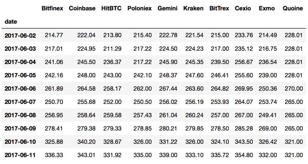
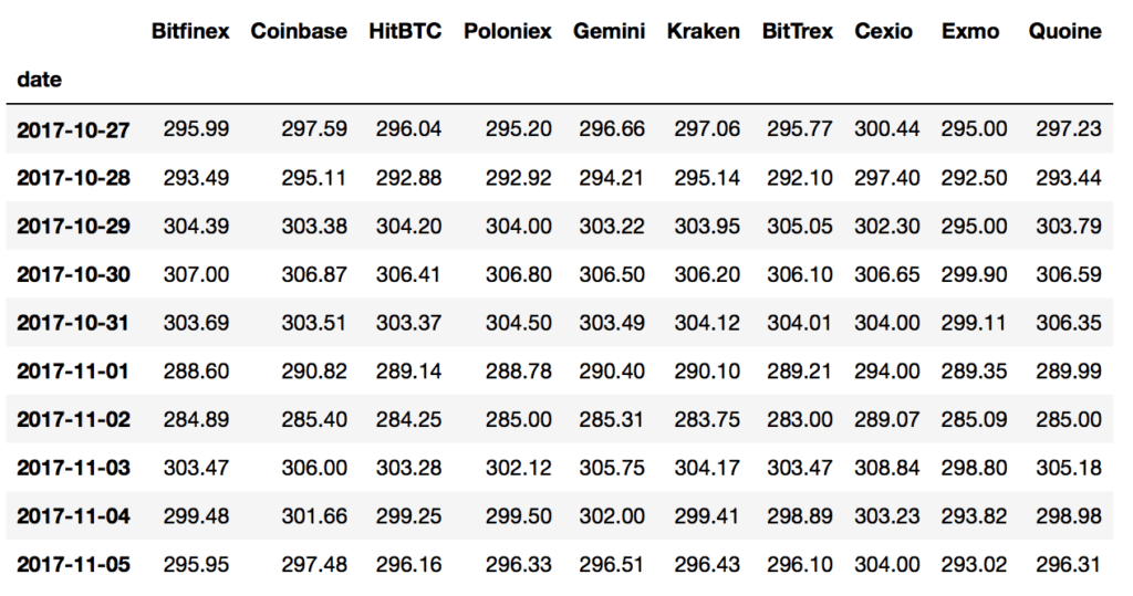
what we can verify by displaying the first and the last ten lines of DataFrame:
print(cp.head(10))
print(cp.tail(10))


Therefore, we have daily close price time-series coming from 10 different markets in our hands. The numbers confirm the noticeable differences among these markets at the close. Now, let’s see how one can pick up a (some) good market(s) for our Stat Arb trading strategy.
4. Average Spread Estimation for ETH/USD among different Markets
By spread, here, I do not mean the distance between Bid and Ask for ETH/USD. Rather than that, given all time-serires, I mean the measurement of the average distance (in USD) between price-series (daily) for the time period covered (Jun 2 till Nov 5, 2018) and supplementing it with one standard deviation, i.e.
dist = []
for i in range(cp.shape[1]):
    for j in range(i):
        if(i != j):
            x = np.array(cp.iloc[:,i], dtype=np.float32)
            y = np.array(cp.iloc[:,j], dtype=np.float32)
            diff = np.abs(x-y)
            avg = np.mean(diff)
            std = np.std(diff, ddof=1)
            dist.append([cp.columns[i], cp.columns[j], avg, std])

dist = sorted(dist, key=lambda x: -x[2])
print("%10s%10s%10s%10s\n" % ("Coin1", "Coin2", "Mean", "Std Dev"))
for e in dist:
    print("%10s%10s%10.5f%10.2f" % (e[0], e[1], e[2], e[3]))
In our case, the code returns the following results:
     Coin1     Coin2      Mean   Std Dev

    Quoine      Exmo  31.18089     38.58
    Quoine     Cexio  31.07745     37.74
    Quoine  Poloniex  30.22300     40.33
    Quoine  Bitfinex  30.10771     40.25
    Quoine   BitTrex  30.05567     40.36
    Quoine  Coinbase  29.90038     40.07
    Quoine    Kraken  29.82280     40.04
    Quoine    HitBTC  29.82038     39.48
    Quoine    Gemini  29.71771     40.15
     Cexio    HitBTC   9.88497      8.28
     Cexio  Poloniex   9.68694      8.26
      Exmo     Cexio   9.58420      5.15
     Cexio   BitTrex   9.57796      8.27
     Cexio  Bitfinex   9.56936      7.96
     Cexio    Gemini   8.57503      8.20
     Cexio    Kraken   8.25248      6.54
     Cexio  Coinbase   7.84471      6.23
      Exmo   BitTrex   6.37057      5.34
      Exmo  Poloniex   6.23357      5.20
      Exmo    HitBTC   6.22764      5.00
      Exmo  Bitfinex   6.12720      5.01
      Exmo    Gemini   6.04459      6.21
      Exmo    Kraken   6.00204      4.35 *
      Exmo  Coinbase   5.74370      4.20
    HitBTC  Coinbase   2.77898      4.38
    Gemini    HitBTC   2.77732      5.61
    Kraken    HitBTC   2.63350      3.89
   BitTrex    Gemini   2.51720      4.78
   BitTrex    Kraken   2.48357      3.18
   BitTrex  Coinbase   2.46280      3.25
    Gemini  Poloniex   2.34541      5.04
    Kraken  Poloniex   2.30720      3.41
  Poloniex  Coinbase   2.27586      3.47
    Kraken  Bitfinex   2.16834      2.73
    Gemini  Bitfinex   2.16121      4.60
  Coinbase  Bitfinex   2.10006      2.81
    Kraken    Gemini   1.91146      5.16
   BitTrex    HitBTC   1.88293      3.52
  Poloniex    HitBTC   1.55051      3.61
    Kraken  Coinbase   1.51592      2.52
    HitBTC  Bitfinex   1.48223      3.33
   BitTrex  Poloniex   1.43484      2.39
   BitTrex  Bitfinex   1.23981      1.92
    Gemini  Coinbase   1.23809      4.75
  Poloniex  Bitfinex   0.68331      1.92
In theory, we want to select two markets with the highest mean spread at the lowest standard deviation (assuming that the distances calculated follow the normal distribution). In practice, given above numbers, you can check all combinations (in the backtest we are going to write below) in order to find out what what really works best.
5. Statistical Arbitrage Trading Strategy for ETH/USD
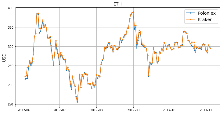
Let me choose Exmo and Kraken exchanges. The mean spread of 6 USD at $1\sigma$ of 4.25 USD gives a lot of hope for good fishing! We start from downloading the corresponding time-series (df1 and df2) followed by their quick visualisation:
market1 = "Exmo"
market2 = "Kraken"

df1 = fetchCryptoOHLC_byExchange(fsym, tsym, market1)
df2 = fetchCryptoOHLC_byExchange(fsym, tsym, market2)

# trim
df1 = df1[(df1.index > "2017-06-01") & (df1.index <= "2017-11-05")]
df2 = df2[(df2.index > "2017-06-01") & (df2.index <= "2017-11-05")]

# checkpoint
print(df1.close.shape[0], df2.close.shape[0])  # both sizes must be equal

# plotting
plt.figure(figsize=(20,10))
plt.plot(df1.close, '.-', label=market1)
plt.plot(df2.close, '.-', label=market2)
plt.legend(loc=2)
plt.title(fsym, fontsize=12)
plt.ylabel(tsym, fontsize=12)
plt.grid()
Every trading strategy requires some boundary conditions. Let’s summarise them all together before coding:
Therefore, we start trading with USD 5,000 on Exmo and Kraken account, respectively. That will allow us to monitor the “cash” level of both accounts after each trade. The full code to perform the backtest would look like this:
# Backtesting Stat Arb trading strategy for ETH/USD at Exmo and Kraken
#  cryptocurrency exchanges

# initial parameters
investment = 10000  # USD
account1, account2 = investment/2, investment/2  # USD
position = 0.5*(investment/2)  # USD

roi = []
ac1 = [account1]
ac2 = [account2]
money = []
pnl_exch1 = []
pnl_exch2 = []

trade = False
n = df1.close.shape[0]  # number of data points

# running the backtest
for i in range(n):
    p1 = float(df1.close.iloc[i])
    p2 = float(df2.close.iloc[i])
    if(p1 > p2):
        asset1 = "SHORT"
        asset2 = "LONG"
        if(trade == False):
            open_p1 = p1  # open prices
            open_p2 = p2
            open_asset1 = asset1
            open_asset2 = asset2
            trade = True
            print("new traded opened")
            new_trade = False
        elif(asset1 == open_asset1):
            new_trade = False  # flag
        elif(asset1 == open_asset2):
            new_trade = True   # flag

    elif(p2 > p1):
        asset1 = "LONG"
        asset2 = "SHORT"
        if(trade == False):
            open_p1 = p1  # open prices
            open_p2 = p2
            open_asset1 = asset1
            open_asset2 = asset2
            trade = True
            print("new traded opened")
            new_trade = False
        elif(asset1 == open_asset1):
            new_trade = False  # flag
        elif(asset1 == open_asset2):
            new_trade = True   # flag

    if(i == 0):
        print(df1.close.iloc[i], df2.close.iloc[i], \
              asset1, asset2, trade, "----first trade info")
    else:
        if(new_trade):

            # close current position
            if(open_asset1 == "SHORT"):
                # PnL of both trades
                pnl_asset1 = open_p1/p1 - 1
                pnl_asset2 = p2/open_p2 -1
                pnl_exch1.append(pnl_asset1)
                pnl_exch2.append(pnl_asset2)
                print(open_p1, p1, open_p2, p2, open_asset1, \
                      open_asset2, pnl_asset1, pnl_asset2)
                # update both accounts
                account1 = account1 + position*pnl_asset1
                account2 = account2 + position*pnl_asset2
                print("accounts [USD] = ", account1, account2)
                if((account1 <=0) or (account2 <=0)):
                    print("--trading halted")
                    break
                # return on investment (ROI)
                total = account1 + account2
                roi.append(total/investment-1)
                ac1.append(account1)
                ac2.append(account2)
                money.append(total)
                print("ROI = ", roi[-1])
                print("trade closed\n")
                trade = False

                # open a new trade
                if(asset1 == "SHORT"):
                    open_p1 = p1
                    open_p2 = p2
                    open_asset1 = asset1
                    open_asset2 = asset2
                else:
                    open_p1 = p1
                    open_p2 = p2
                    open_asset1 = asset1
                    open_asset2 = asset2
                trade = True
                print("new trade opened", asset1, asset2, \
                      open_p1, open_p2)

            # close current position
            if(open_asset1 == "LONG"):
                # PnL of both trades
                pnl_asset1 = p1/open_p1 -1
                pnl_asset2 = open_p2/p2 - 1
                pnl_exch1.append(pnl_asset1)
                pnl_exch2.append(pnl_asset2)
                print(open_p1, p1, open_p2, p2, open_asset1, \
                      open_asset2, pnl_asset1, pnl_asset2)
                # update both accounts
                account1 = account1 + position*pnl_asset1
                account2 = account2 + position*pnl_asset2
                print("accounts [USD] = ", account1, account2)
                if((account1 <=0) or (account2 <=0)):
                    print("--trading halted")
                    break
                # return on investment (ROI)
                total = account1 + account2
                roi.append(total/investment-1)
                ac1.append(account1)
                ac2.append(account2)
                money.append(total)
                trade_pnl.append(pnl_asset1+pnl_asset2)
                print("ROI = ", roi[-1])
                print("trade closed\n")
                trade = False

                # open a new trade
                if(open_asset1 == "SHORT"):
                    open_p1 = p1
                    open_p2 = p2
                    open_asset1 = asset1
                    open_asset2 = asset2
                else:
                    open_p1 = p1
                    open_p2 = p2
                    open_asset1 = asset1
                    open_asset2 = asset2
                new_trade = False
                trade = True
                print("new trade opened:", asset1, asset2, \
                      open_p1, open_p2)

        else:
            print("   ",df1.close.iloc[i], df2.close.iloc[i], \
                  asset1, asset2)
An exemplary trading log you should recover based on data sample selected above commences with:
new traded opened
214.49 221.54 LONG SHORT True ----first trade info
    216.75 224.23 LONG SHORT
    236.54 245.35 LONG SHORT
    239.0 247.6 LONG SHORT
    250.36 263.6 LONG SHORT
    253.74 256.19 LONG SHORT
    249.41 260.24 LONG SHORT
    269.0 279.85 LONG SHORT
214.49 326.42 221.54 326.0 LONG SHORT 0.5218425101403328 -0.32042944785276073
accounts [USD] =  6304.606275350832 4198.926380368098
ROI =  0.05035326557189301
trade closed

new trade opened: SHORT LONG 326.42 326.0
326.42 332.0 326.0 333.1 SHORT LONG -0.016807228915662553 0.021779141104294464
accounts [USD] =  6262.588203061676 4253.374233128834
ROI =  0.05159624361905091
trade closed

new trade opened LONG SHORT 332.0 333.1
332.0 332.0 333.1 333.1 LONG SHORT 0.0 0.0
accounts [USD] =  6262.588203061676 4253.374233128834
ROI =  0.05159624361905091
trade closed

new trade opened: LONG SHORT 332.0 333.1
332.0 390.0 333.1 385.0 LONG SHORT 0.17469879518072284 -0.1348051948051947
accounts [USD] =  6699.3351910134825 3916.3612461158473
ROI =  0.06156964371293294
trade closed

new trade opened: SHORT LONG 390.0 385.0
    393.2 386.13 SHORT LONG
    369.41 347.24 SHORT LONG
    357.3 345.99 SHORT LONG
    365.81 354.17 SHORT LONG
    370.61 368.95 SHORT LONG
    357.0 349.5 SHORT LONG
    359.82 356.48 SHORT LONG
    358.03 348.5 SHORT LONG
    334.0 324.48 SHORT LONG
    325.95 321.6 SHORT LONG
    334.0 325.5 SHORT LONG
    317.47 302.15 SHORT LONG
    295.0 277.0 SHORT LONG
    264.0 254.49 SHORT LONG
390.0 280.93 385.0 283.66 SHORT LONG 0.38824618232299857 -0.26322077922077913
accounts [USD] =  7669.950646820979 3258.3092980638994
ROI =  0.09282599448848772
trade closed

...
In the first trade we open a long position at Exmo at price of 214.49 and a short position at Kraken at 221.54. After 8 days, there has been a new trading signal generated what caused to close both positions. The close price at Exmo was 326.42 so we made a profit +52.18% while the concurrent short position at Kraken closed with a loss of 32.04% because of ETH/USD rose from 221.54 up to 326.0. In result, the cash at Exmo account went up from 5,000 to 6,304.61 while at Kraken account down from 5,000 to 4,198.93 (=5000 – 0.3204$\times$2500). A new trade has been opened with a short position at Exmo and long position at Kraken, etc.
Having the backtest code, there are many places you can take it and analyse its variants. If you build-in the commission fee structure, you may find the difference in profits with and without the fees. I strongly encourage to experiment with it. Who knows… maybe you will become a millionaire too?! :-)
Just to assist with the understanding of some numbers we captured along the backtest (see all Python lists; lines #163-168), first let’s have a look at the cash level in both accounts:
plt.figure(figsize=(12,7))

plt.subplot(2,3,1)
plt.plot(ac1)
plt.title("Exmo: Cash Level")
plt.xlabel("Trade No."); plt.ylabel("USD")
plt.grid()
plt.xlim([0, len(money)])
plt.ylim([0, 14001])

plt.subplot(2,3,2)
plt.plot(ac2)
plt.title("Kraken: Cash Level")
plt.xlabel("Trade No."); plt.ylabel("USD")
plt.grid()
plt.xlim([0, len(money)])
plt.ylim([0, 14001])

plt.subplot(2,3,3)
plt.plot(np.array(money))
plt.title("Total Cash")
plt.xlabel("Trade No."); plt.ylabel("USD")
plt.grid()
plt.xlim([0, len(money)])
plt.ylim([investment, 14000])

plt.tight_layout()
plt.savefig('cashlevels.png', bbox_inches='tight')

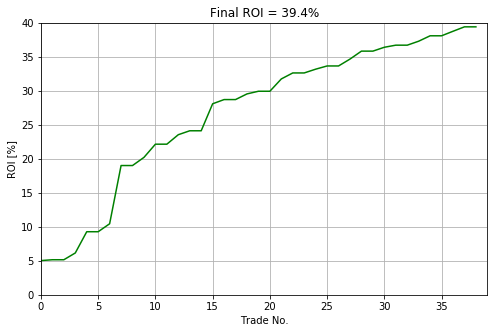
These charts indicate that within our Stat Arb strategy the performance of trades at Exmo was much much better than at Kraken. Only the final ca. 10 trades at Kraken brought some profits. Both characteristics have their conclusion as presented on the third chart: Total Cash.
In other words, after 5 months of running the strategy, we ended up with a nice +39.4% return on our initial investment of USD 10,000, i.e.
plt.figure(figsize=(8,5))
plt.plot(np.array(roi)*100, 'g')
plt.xlabel("Trade No.");
plt.ylabel("Equity Growth [%]")
plt.title("ROI = %f.2%%" % (100*roi[-1]))
plt.xlim([0, len(money)])
plt.ylim([0, 40])
plt.grid()
plt.savefig('roi.png', bbox_inches='tight')
Final Note
Greed is good. Use this algo wisely! Don’t buy a jet. Instead, make your wife happy. Tiffany would do the job… :-)


7 comments
Hey very cool blog!! Man .. Beautiful .. Wonderful .. I will bookmark your website and
take the feeds additionally? I’m satisfied to search out numerous useful info right here within the post, we need work out more
techniques on this regard, thanks for sharing. . . . . .
Hi nice article. trade_pnl is not declared in your code !
the only thing you are missing, is the delirious cost to trade cryptos on those new pseudo exchanges…ROI < 0
Hi Pawel,
Very nice article! One tip can be using the request session to leverage the keep-alive connection.
s = requests.session()
trying something like:
response = s.get(url)
instead of
response = request.get(url)
Best,
Ronaldo
when running
====================
# Select Top 10 Cryptocurrency Markets by their volume
markets = [e[0] for e in vol][0:10]
print(markets)
==================
i am getting this (which is not as shown above):
Bitfinex 220700.34
[‘Bitfinex’, ‘Coinbase’, ‘Gemini’, ‘Poloniex’, ‘HitBTC’, ‘Kraken’, ‘BitTrex’, ‘Cexio’, ‘Exmo’, ‘Quoine’]
Coinbase 144549.34
[‘Bitfinex’, ‘Coinbase’, ‘Gemini’, ‘Poloniex’, ‘HitBTC’, ‘Kraken’, ‘BitTrex’, ‘Cexio’, ‘Exmo’, ‘Quoine’]
Gemini 44508.90
[‘Bitfinex’, ‘Coinbase’, ‘Gemini’, ‘Poloniex’, ‘HitBTC’, ‘Kraken’, ‘BitTrex’, ‘Cexio’, ‘Exmo’, ‘Quoine’]
Poloniex 37787.74
[‘Bitfinex’, ‘Coinbase’, ‘Gemini’, ‘Poloniex’, ‘HitBTC’, ‘Kraken’, ‘BitTrex’, ‘Cexio’, ‘Exmo’, ‘Quoine’]
I will be happy if you could assist me what did i do wrong. thanks!
Are your “prices” mid-point quotes, or trades? If trades, are you sure you are not simply fitting to stale trade noise? I’d wager this entire strategy is untradeable.
Hello Pawel,
Very good article :)
I think you are missing declare trade_pnl = [] array in your code !
Regards
Ludo.