How to Predict Bitcoin Price with Deep Learning LSTM Network

You can’t predict the future unless you have a crystal ball but you can predict Bitcoin price in next time step if you have a right tool and enough confidence in your model. With the development of a new class of forecasting models employing Deep Learning neural networks, we gained new opportunities in foreseeing near future.

A rebirth of Long Short Term Memory (LSTM) artificial recurrent neural network (RNN) architecture, originally proposed in 1997 by Sepp Hochreiter and Jürgen Schmidhuber (reference), sparked a new wave of optimism in guessing the future better by studying the past deeper. No wonder why. With a specific design of the LSTM unit, the analysis of time-series’ data points and their sequential relationships gave a hope that we could train the network to be able to estimate next movement by what we have seen before (train set). However, since it does not always pay off to rely solely on the past, our predictions could be close to reality (test set), indeed. Of course, the goal is to push the error of prediction down to zero. Wouldn’t it be wonderful?

Is it difficult? How many different elements of this landscape we need to control to make the neural network’s predictions close enough to real observations? Within this dedicated series of articles devoted to hourly Bitcoin (BTC) close price prediction, I will try to present the whole complexity in construction and fine tuning of the Deep Learning network, here employing the LSTM model.

We will start differently, however. Namely, in this post, first, I will present a full Python code as a benchmark code and in the following posts, we will analyse in depth all elements of the process and their impact on the final result. You will learn how a small change at any stage can spoil or improve predictions. And trust me on that, everything matters here! A selection of train and test data sets, a number of features, a selection and quality of these features, feature correlation and co-integration, input data pre-processing, the LSTM network design, a number of hidden layers, a number of epochs, a size of batches, a selection of optimiser – just to name few.

If you think that a construction of a successful Deep Learning network for time-series prediction is just a walk in the park, stay with me. It will be a long walk… And one more thing. Don’t trust your eyes. What you will see at the end, is not how it should be. Intrigued enough? Keep walking…

1. Objective: Predict Bitcoin Price

Design and train the LSTM network fuelled by input/train data (multiple cryptocurrency time-series with 60 min resolution) in order to predict Bitcoin price in an hour such to achieve minimal Root Mean Squared Error (RMSE) between true and predicted prices over the entire test data sample.

2. Data Selection

We would like to make a prediction of the BTC/USD close price based on close price-series of three cryptocurrencies, i.e. Ethereum (ETH/USD), Tezos (XTZ/USD), and Litecoin (LTC/USD), with a possibility of including BTC/USD data as well. The prediction will be one-step-ahead which means 1-hour ahead in our case and the training set will be based on close prices of aforementioned cryptocurrencies an hour and two hours earlier.

To download the cryptocurrency time-series for all four coins, we will use the resources of cryptocompare.com and the function of getMultipleCrypoSeries for that purpose. This function is a part of the ccrypto library and it will be available soon as an integrated part of my book Cryptocurrencies with Python.

# How to Predict Bitcoin Price with Deep Learning LSTM Network: (1) The Model
#
# (c) 2020 by Pawel Lachowicz, PhD

from ccrypto import getMultipleCrypoSeries

import numpy as np
import pandas as pd
import matplotlib.pyplot as plt
from IPython.display import display, display_html, HTML


# --Data Selection

ccpairs = ['BTCUSD', 'ETHUSD', 'XTZUSD', 'LTCUSD']
df = getMultipleCrypoSeries(ccpairs, freq='h', exch='Coinbase', 
                            start_date='2019-08-09 13:00', end_date='2020-03-13 23:00')

display(df)

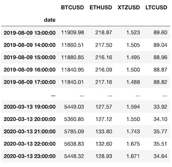
These time-series we can visually compare in one chart after applying normalisation as follows:

from sklearn.preprocessing import MinMaxScaler

scaler = MinMaxScaler(feature_range=(0, 1))
sdf_np = scaler.fit_transform(df)  # note: scaler converts df into numpy array
sdf = pd.DataFrame(sdf_np, columns=df.columns, index=df.index)

plt.figure(figsize=(12,6))
plt.grid()
plt.plot(sdf)
plt.legend(sdf.columns)

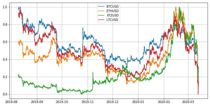
A motivation for the selection of Litecoin and Ethereum is their pretty high correlation with Bitcoin regardless the number of hours taken into account. We can diagnose this by measuring the average linear correlation over the rolling window in a function of rolling window size:

blue, orange, red = '#1f77b4', '#ff7f0e', '#d62728'  # color codes

plt.figure(figsize=(12,4))
plt.grid()

avg_corr1, avg_corr2, avg_corr3 = list(), list(), list()

# average correlation for increasing rolling window size
for win in range(3, 72):  # hours
    avg_corr1.append(df.ETHUSD.rolling(win).corr(df.BTCUSD) 
                     .replace([np.inf, -np.inf], np.nan).dropna().mean())
    avg_corr2.append(df.XTZUSD.rolling(win).corr(df.BTCUSD) 
                     .replace([np.inf, -np.inf], np.nan).dropna().mean())
    avg_corr3.append(df.LTCUSD.rolling(win).corr(df.BTCUSD) 
                     .replace([np.inf, -np.inf], np.nan).dropna().mean())
    
plt.plot(range(3, 72), avg_corr1, '.-', color=blue, label='ETH vs BTC')
plt.plot(range(3, 72), avg_corr2, '.-', color=orange, label='XTZ vs BTC')
plt.plot(range(3, 72), avg_corr3, '.-', color=red, label='LTC vs BTC')

plt.legend()
plt.xlabel('Rolling Window Length [hours]', fontsize=12)
plt.ylabel('Average Correlation', fontsize=12)

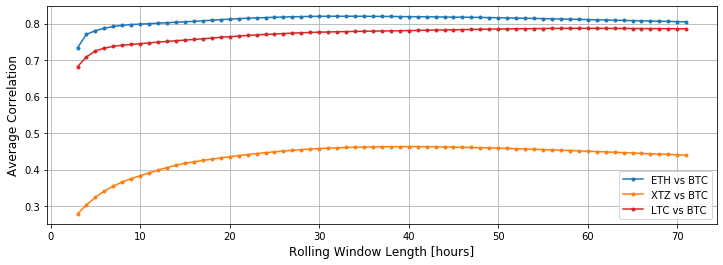
Tezos appears to be less correlated with Bitcoin but purposely I will include and leave it in the input set.

3. Feature Engineering

The establishment of the train dataset seems to be one of the major player in the game. We select and provide the bulk of past observations or data experience as a learning input. Intuitively, the more we deliver the better results we expect to receive. Not exactly, but that’s a good starting point.

We distinguish features and labels. By labels (or a single label) we will understand the values we want to predict. Say, the Bitcoin price in an hour, two, three, etc. (labels) or just a price in an hour (label).

In the train sample, a label is used for training. We provide a range of features and show computer the associated label. For example, if our set of features are the prices of three cryptocurrencies an hour ago $(t-1)$ and two hours ago $(t-2$) as in our Objective and the label is the Bitcoin price in an hour $(t)$, we want our computer to learn the relationship between the precedent values of other cryptocurrency prices and the “expected” Bitcoin price. But why? Simply for a reason that when a similarity occurs for new, never seen, cryptocurrency price-series or test sample, based on the past learning experience, the prediction of Bitcoin price should be more accurate. Well, that’s the goal of learning. If you touch a hot frying pan with a bare hand, you will learn not to touch it again the same way.

Let’s assume we are correct when it comes to such reasoning as above. If so, we can have a look at features and labels preparation process. To begin, let’s equip ourselves with a handy function that allows to display two DataFrames side by side in a one row:

def displayS(dfs:list, captions:list, space=5):
    """Display tables side by side to save vertical space
    Input:
        dfs: list of pandas.DataFrame
        captions: list of table captions
    """
    output = ""
    combined = dict(zip(captions, dfs))
    for caption, df in combined.items():
        output += df.style.set_table_attributes("style='display:inline'") 
                  .set_caption(caption)._repr_html_()
        output += space * "xa0xa0xa0"
    display(HTML(output))

Next, we’re going to use an another function from ccrypto library (reference) which simply takes raw input time-series, allows us to specify which one should be taken as the label (in our case it is BTC/USD), and how many hour lags we would like to use in order to generate a set of features. Analyse what follows:

# --Features and Label Engineering

label = 'BTCUSD'

from ccrypto import get_features_and_labels

out_X, _, out_y, _ = get_features_and_labels(df, label, 
                                             timesteps=2, 
                                             exclude_lagged_label=False, 
                                             train_fraction=0  # no train/test split
                                            )

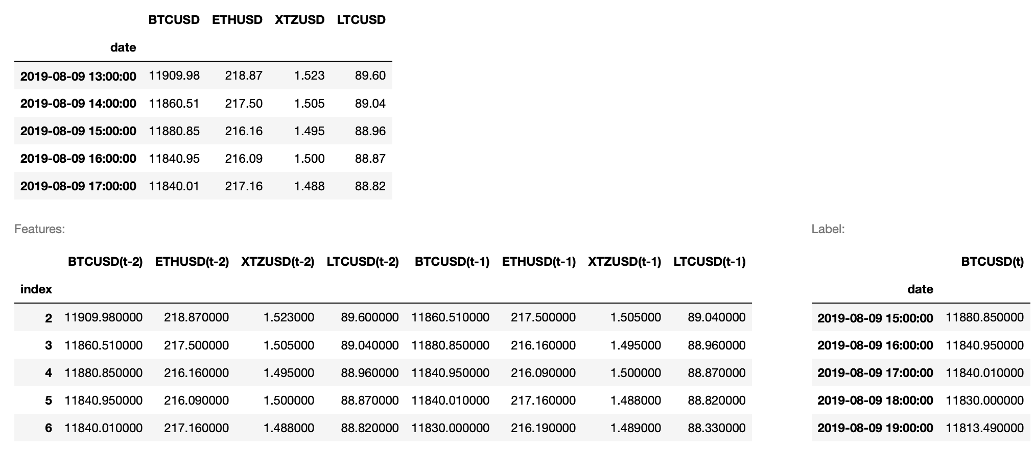
display(df.head())
displayS([out_X.head(), out_y.head()], ['Features:', 'Label:'])

The code returns:

Again, the logic of feeding the beast is simple here. If we want to predict the Bitcoin price of 11840.01 USD we are going to use the data of all cryptocurrencies an hour $(t-1)$ and two hours ago $(t-2)$.

Train / Test Sample Split

The same function can be used to split the input data into train and test samples. All we have to do is to decide what fraction of time-series (counting from their beginning) we are going to use for training of the LSTM network. I will assume it will be $95%$:

# train/test sample

train_fract = 0.95

train_X, train_y, test_X, test_y = get_features_and_labels(df, label, 
                                                           timesteps=2, 
                                                           exclude_lagged_label=False, 
                                                           train_fraction=train_fract
                                                          )

# check dimensions of arrays
print(train_X.shape, train_y.shape, test_X.shape, test_y.shape)

(4972, 8) (4972, 1) (260, 8) (260, 1)

Therefore, we will be using 4972 observations times 8 features for training, and the out-of-sample test will be conducted on 260 new Bitcoin close prices. If we can predict these 260 values very accurately, we can start our own hedge fund right away!

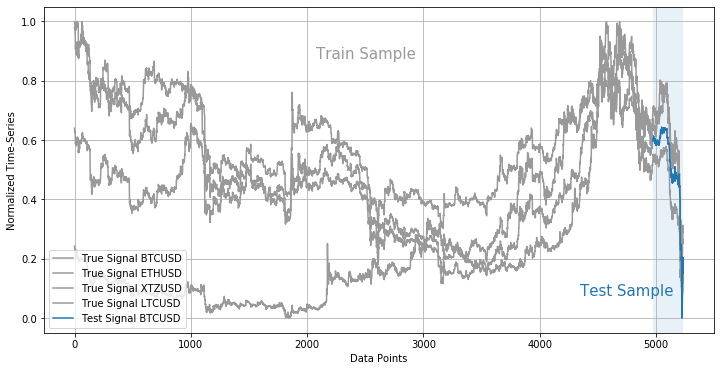
The train/test data samples can be illustrated as follows:

# visualise train/test samples

data_size = df.shape[0]
train_size = int(data_size * train_fract)
test_size = data_size - train_size

plt.figure(figsize=(12,6))
plt.grid()

for cn in sdf.columns:
    plt.plot(np.arange(train_size+test_size), sdf[cn], color=grey, 
            label='True Signal ' + cn)  # sdf[cn].iloc[:train_size]

plt.plot(np.arange(train_size, train_size+test_size), sdf[label].iloc[train_size:], 
            color=blue, label='Test Signal ' + label)

plt.axvspan(train_size, test_size+train_size, facecolor=blue, alpha=0.1)
plt.annotate("Train Sample", xy=(2075, 0.875), fontsize=15, color=grey)
plt.annotate("Test Sample", xy=(4350, 0.075), fontsize=15, color=blue)
plt.xlabel("Data Points")
plt.ylabel("Normalized Time-Series")
plt.legend(loc=3)

This step in Feature and Label Engineering process is quite important so let’s pause here for a second. By studying the patterns of time-series of train sample, one can notice a huge variety. Keeping in mind that learning will be based over 3 hour intervals, intuitively, the abundance of structures should cover a lot of sequential relationships between lagged data points and target (label) Bitcoin price. Therefore, both sudden spike in underlying price-series as well as price falling down should matter. How much? That depends on recurrent learning process within the LSTM network which we’re going to define now.

4. LSTM Network for Bitcoin

This won’t be difficult. I will design a simple architecture of the network. Don’t worry if you don’t understand the details, I will explain the RNN LSTM engine-at-work in the following parts in this series. For now, it is sufficient to know that our LSTM network will be composed of $8times 5 = 40$ units and one Dropout layer. The output is a Dense layer (one cell) to return predicted Bitcoin price.

We will use of TensorFlow 2.1.x (TF) to construct the network. You can find all information on TF integration with your Python environment in my previous post Setup of Keras and TensorFlow 2.1+ for Deep Learning in Python.

TF makes use of Keras-based wrapper which requires the input data to come in a specific format. First we need to re-use get_features_and_labels function to return train and test samples as NumPy arrays instead of pandas’ DataFrame (as we have done it above), and next to use reshape function to prepare the data for TF:

# --LSTM

train_fract = 0.95
timesteps = 2
train_X, train_y, test_X, test_y = get_features_and_labels(sdf, label, 
                                                           timesteps=timesteps, 
                                                           train_fraction=train_fract, 
                                                           as_np=True,
                                                           exclude_lagged_label=False)

# reshape input to be 3D [samples, timesteps, features]
train_X = train_X.reshape((train_X.shape[0], 1, train_X.shape[1]))
test_X  = test_X.reshape((test_X.shape[0], 1, test_X.shape[1]))

print(train_X.shape, train_y.shape, test_X.shape, test_y.shape)

(4972, 1, 8) (4972, 1) (260, 1, 8) (260, 1)

Having the input data ready, we can design the network:

import tensorflow as tf

# use seed for reproducability of results
tf.random.set_seed(7)

# model's parameters
dropout_fraction = 0.1
units = 8*5
ishape = train_X.shape[1], train_X.shape[2]

model = tf.keras.models.Sequential()
model.add(tf.keras.layers.LSTM(units, return_sequences=True, input_shape=ishape))
model.add(tf.keras.layers.Dropout(dropout_fraction))
model.add(tf.keras.layers.TimeDistributed(tf.keras.layers.Dense(1)))

# compile using mean-squared-error loss function
model.compile(loss='mse', optimizer='adam')

# display network's simplified architecture
print(model.summary())

Model: "sequential_1"
_________________________________________________________________
Layer (type)                 Output Shape              Param #   
=================================================================
lstm_2 (LSTM)                (None, 1, 40)             7840      
_________________________________________________________________
dropout_2 (Dropout)          (None, 1, 40)             0         
_________________________________________________________________
time_distributed_2 (TimeDist (None, 1, 1)              41        
=================================================================
Total params: 7,881
Trainable params: 7,881
Non-trainable params: 0
_________________________________________________________________
None

The training of our LSTM network can be executed by the following fitting function:

# train the network using input dataset
n_epochs = 3000
batch_size = train_X.shape[0]//5

history = model.fit(train_X, train_y, epochs=n_epochs, batch_size=batch_size, 
                    validation_data=(test_X, test_y), verbose=0, shuffle=False)

The number of epochs simply means how long we want train the network where the batch size is the size of data points used in training (more on these parameters in next posts). If verbose is set to zero, the model.fit function won’t print the progress in fitting. For $verbose=1$ we can preview the process as it runs:

Train on 4972 samples, validate on 260 samples
Epoch 1/3000
4972/4972 [=================] - 1s 227us/sample - loss: 0.2698 - val_loss: 0.1500
Epoch 2/3000
4972/4972 [=================] - 0s 5us/sample - loss: 0.2131 - val_loss: 0.1028
Epoch 3/3000
4972/4972 [=================] - 0s 5us/sample - loss: 0.1629 - val_loss: 0.0638
Epoch 4/3000
4972/4972 [=================] - 0s 4us/sample - loss: 0.1188 - val_loss: 0.0338
Epoch 5/3000
4972/4972 [=================] - 0s 5us/sample - loss: 0.0829 - val_loss: 0.0135
...
Epoch 2998/3000
4972/4972 [=================] - 0s 4us/sample - loss: 1.5742e-04 - val_loss: 3.5775e-04
Epoch 2999/3000
4972/4972 [=================] - 0s 5us/sample - loss: 1.5482e-04 - val_loss: 3.4328e-04
Epoch 3000/3000
4972/4972 [=================] - 0s 4us/sample - loss: 1.4600e-04 - val_loss: 3.8304e-04

In order to visualise the evolution of loss function, we may use the following code:

plt.figure(figsize=(12,2))
plt.grid()
plt.plot(history.history['loss'], label='train')
plt.plot(history.history['val_loss'], label='test')
plt.ylabel('Loss')
_ = plt.legend()

plt.figure(figsize=(12,2))
plt.grid()
plt.ylabel('Loss')
plt.semilogy(history.history['loss'], label='train')
plt.semilogy(history.history['val_loss'], label='test')
_ = plt.legend()

where it’s helpful to compare the plot of the same function with linear and logarithmic scale of the y-axis:

These plots are a very useful diagnostic tool in the process of assessing whether the model underfits or overfits the data. We will come back to this, soon.

5. Prediction of Bitcoin Close Price in Test Sample

TF allows to make the prediction of the model on test sample with a single line of code. To test the goodness of fit (predicted Bitcoin prices vs real values), we will use the mean squared error regression loss (MSE) metric:

yhat = model.predict(test_X)  # make a prediction
yorg = sdf[label].iloc[train_X.shape[0]+timesteps:]  # true (test) signal

# reshape both arrays to NumPy vectors
yhat_f = yhat.flatten()
yorg_f = yorg.values.flatten()

# calculate mean squared error regression loss 
from sklearn.metrics import mean_squared_error
rmse = np.sqrt(mean_squared_error(yhat_f, yorg_f))
print('Test MSE: %.5f' % rmse)

Test MSE: 0.01957

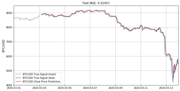
What does it mean? For now I can only tell you that this error measure is the lowest I have obtained after few hours playing the We can illustrate the final fit over test sample as follows:

# convert prediction of BTC close price back to USD
z = np.zeros((test_size-timesteps, 4))
z[:,0] = yhat_f
yhat_inv = scaler.inverse_transform(z)[:,0]
yorg_inv = scaler.inverse_transform(sdf)[:,0]  # entire time-series

# plot prediction vs real BTC close price
plt.figure(figsize=(12,6))
plt.grid()
plt.plot(df.index[0:train_size], yorg_inv[:train_size], '-', color=grey, 
         label=label+' True Signal (train)')
plt.plot(df.index[train_size+2:], yorg_inv[train_size+2:], '-', color=blue, 
         label=label+' True Signal (test)')
plt.plot(df.index[train_size+2:], yhat_inv, '-',  color=red, label=label+ 
         ' Close Price Prediction')

plt.title('Test MSE: %.5f' % rmse)
plt.ylabel('BTC/USD', fontsize=12)
plt.xlim([pd.to_datetime('2020-03-01'), df.index[-1]])
plt.ylim([4000, 9500])
_ = plt.legend(loc=3)

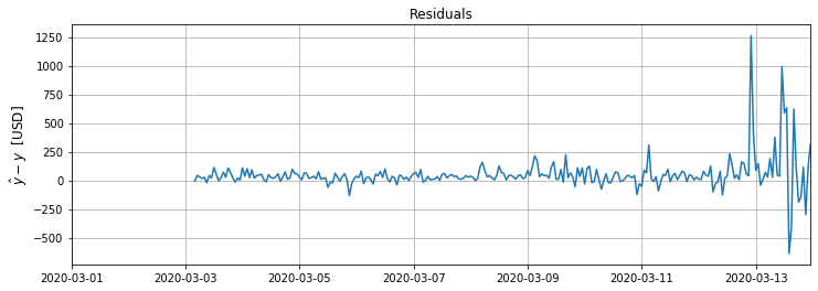
Is it a good fit? Best way to assess that is by plotting the residual signal, i.e. the difference between predicted and actual Bitcoin close prices:

# inspect visually residuals
btc = yorg_inv[train_size+2:]  # true BTC close price
btc_hat = yhat_inv  # predicted BTC close price

plt.figure(figsize=(12,4))
plt.grid()
res =  btc_hat - btc
plt.plot(df.index[train_size+2:], res)
plt.title('Residuals')
plt.xlim([pd.to_datetime('2020-03-01'), df.index[-1]])
plt.savefig("/Users/pawel/Desktop/resid.png", bbox_inches='tight')

This chart reveals a lot. First of all, we can see that RNN LSTM network cannot cope with predicting a sudden price drops as we have seen in BTC prices during recent cryptocurrencies sell-off powered by fears related to coronavirus (notice ca. 1250 USD high spike). Before that events, it handles predictions much better with deviation from real price somewhere between 0 and 150 USD (till 2020-03-07) and between -50 and 250 USD after that date (the beginning of the oil crisis).

In next part, we will dive into model improvement process starting from in-depth analysis of all input time-series. Stay tuned!