Cryptocurrency Price Tracking of Bitcoin Gains since its 3rd Halving

The Bitcoin’s 3rd halving was the most anticipated event this year. This a moment when a reward for all Bitcoin block miners is cut by half. It happens every 4 years or every 210,000 blocks on the Bitcoin blockchain. The previous two halving events took place in 2012 and 2016, respectively. Before the 1st halving, miners were rewarded with 50 BTC and after that only with 25 BTC per block. After the 2nd halving in July 2016, the miners could count solely on 12.5 BTC per block reward.

The 2020 Bitcoin halving were expected to take place on May 12, however due to the speed of the network is was recorded on May 11, ca. 21:23 CET (block #630000). You can quickly check that indeed for mining the precedent block you could be rewarded with 12.5 BTC whereas the next block mined offers 6.25 BTC per block. This will be the case for next 1500+ days as we speak and you can track the countdown to 2024 Bitcoin halving e.g. here.

The analysis of Bitcoin prices gains following the past two halving events seems to follow so called Stock-to-Flow model (S2F) which considers a tandem of increasing Bitcoin prices in relation to the shrinking Bitcoin supply every 4 years. If the history is meant to repeat this time again, then buy heaps of BTC, hold on, retire in two years. It’s not my financial advice, it’s just a speculation on what might happen.

Nevertheless, it’s good to have a piece of code which could be run from time to time to check the actual Bitcoin price statistics since its 3rd halving event. Let me put few lines in Python to generate a quick summary.

# Tracking Bitcoin Gains since its 3rd Halving in 2020 using Python
#
# (c) 2020 QuantAtRisk.com
# by Pawel Lachowicz

import ccrypto as cc

import numpy as np
import pandas as pd
import matplotlib.dates as mdates
from IPython.display import display
import matplotlib.pyplot as plt

# color codes
grey7 = (.7, .7, .7)


# historical BTCUSD timeseries including a timestemp of the 3rd BTC halving
halving_ts = pd.read_pickle('halving2020.df')
halving = halving_ts[halving_ts.index == pd.to_datetime('2020-05-11 21:23')]

# fetch recent 7-day BTCUSD timeseries with 1-min sampling
now = cc.getCryptoSeries('BTC', freq='m', ohlc=False, exch='Coinbase')
now = now[now.index == now.index[-1]]

Here, we use already-saved historical 1-min BTC time-series starting on 2020-05-11 (download it from here). This is followed by fetching from CryptoCompare.com the most recent BTC price-series with 1-min resolution, too.

Given required input time-series, we construct a summary DataFrame including a couple of key quantities:

# create summary statistics in a single DataFrame

# merge data
gain = pd.concat([halving, now])

# overall BTCUSD gain or loss
gain_pct = np.round(100*(now.values[0][0]/halving.values[0][0]-1),2)
gain.loc[gain.shape[0]+1] = [gain_pct]
gain.rename(index = {gain.index[-1] : "Curent Gain or Loss (%)"}, inplace=True)

# add a blank row
gain.loc[gain.shape[0]+1] = ""
gain.rename(index = {gain.index[-1] : ""}, inplace=True) # add a blank row

# calculate the rates
tday = (gain.index[1] - gain.index[0]) / pd.Timedelta('1 days')
thrs = (gain.index[1] - gain.index[0]) / pd.Timedelta('1 hour')
gain_usd = gain.iloc[1] - gain.iloc[0]
highest = halving_ts.max()  # highest BTC reached
peak_gain = (highest[0] / halving.values[0][0] - 1) * 100
dd = 100*(now.values[0][0] / highest - 1); dd = dd.values  # drawdown
ddd = ((now.index - halving_ts.index[np.argmax(halving_ts)]) 
 / pd.Timedelta('1 days'))[0]  # drawdown duration

# add to DataFrame
gain.loc[gain.shape[0]+1] = [np.round(highest,2)[0]]
gain.rename(index = {gain.index[-1] : "Peak Price"}, inplace=True)
gain.loc[gain.shape[0]+1] = [np.round(peak_gain,2)]
gain.rename(index = {gain.index[-1] : "Peak Gain (%)"}, inplace=True)
gain.loc[gain.shape[0]+1] = [np.round(dd,2)[0]]
gain.rename(index = {gain.index[-1] : "Drawdown from Peak Price (%)"}, inplace=True)
gain.loc[gain.shape[0]+1] = [np.round(ddd,2)]
gain.rename(index = {gain.index[-1] : "Drawdown Duration (days)"}, inplace=True)
gain.loc[gain.shape[0]+1] = ""
gain.rename(index = {gain.index[-1] : ""}, inplace=True)
gain.loc[gain.shape[0]+1] = [np.round(tday,2)]
gain.rename(index = {gain.index[-1] : "Days since 3rd Halving"}, inplace=True)
gain.loc[gain.shape[0]+1] = ""
gain.rename(index = {gain.index[-1] : ""}, inplace=True)
gain.loc[gain.shape[0]+1] = "Mean Gain Rates"
gain.rename(index = {gain.index[-1] : ""}, inplace=True)
gain.loc[gain.shape[0]+1] = [np.round((gain_usd/tday)[0],2)]
gain.rename(index = {gain.index[-1] : "USD/day"}, inplace=True)
gain.loc[gain.shape[0]+1] = [np.round((gain_pct/tday),2)]
gain.rename(index = {gain.index[-1] : "%/day"}, inplace=True)
gain.loc[gain.shape[0]+1] = [np.round((gain_usd/thrs)[0],2)]
gain.rename(index = {gain.index[-1] : "USD/hour"}, inplace=True)
gain.loc[gain.shape[0]+1] = [np.round((gain_pct/thrs),2)]
gain.rename(index = {gain.index[-1] : "%/hour"}, inplace=True)

display(gain)

In this moment of writing, which is only 2.8 days after the 3rd Bitcoin halving, the price is up by $+14\%$! Here are details returned by the code:

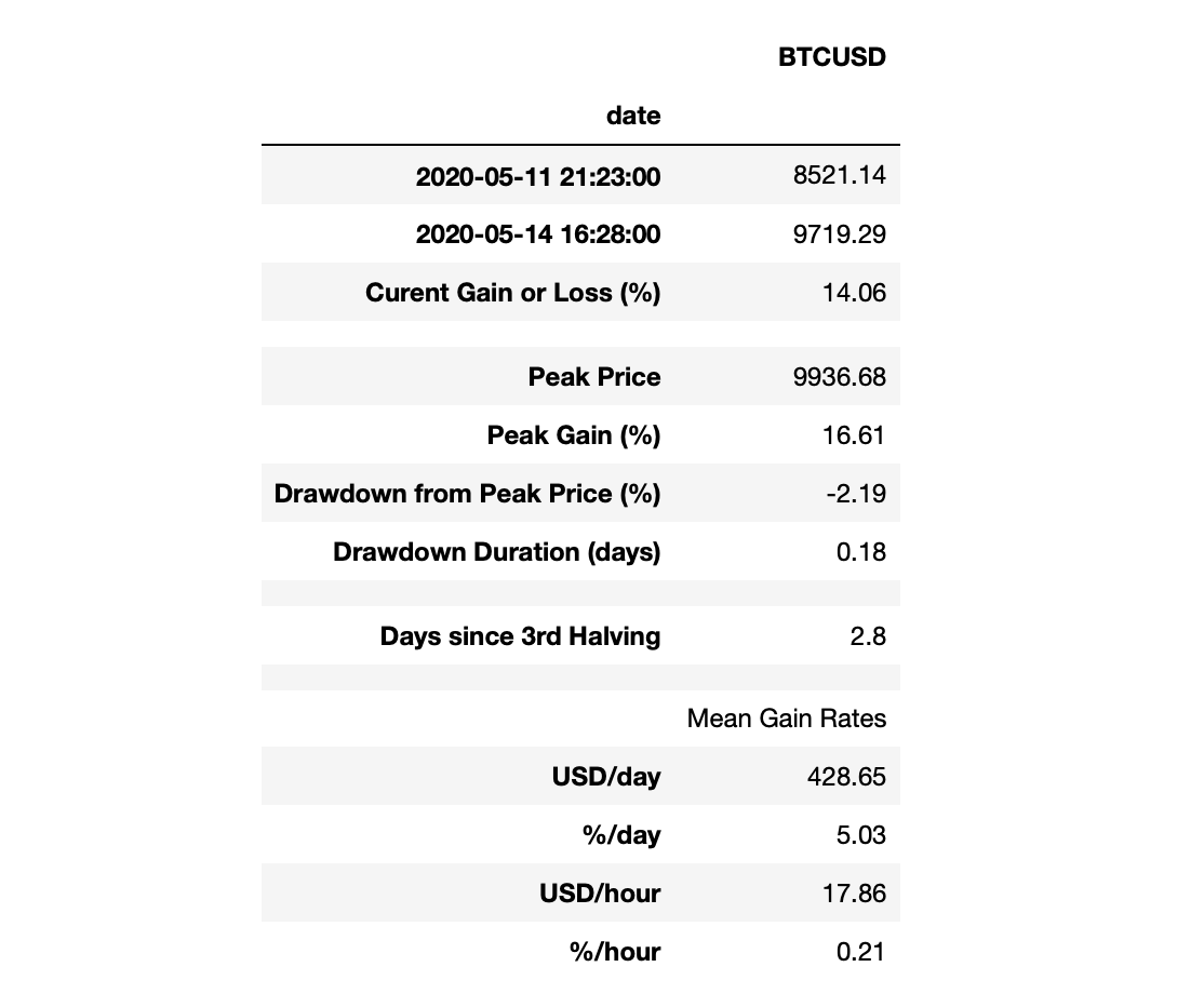
An appealing take-away from this table is the average daily gain rate. Assuming you own only 1 BTC in your portfolio, since the evening of 2020-05-11, you’ve been earning ca. 400 USD per day or 18 USD per hour! Not so bad investment! If only these rates could be maintained at the same level, you could earn your very first million of dollars in 6.8 years from now (that would include 2024 halving, too). Of course, this is a super optimistic scenario but shows that it’s possible to become rich. Just own 10 BTC now and put your faith in S2F model.

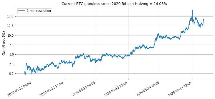
To complete the above code, let’s use the data for the final visualisation:

btc_m = halving_ts[halving_ts.index >= '2020-05-11 21:21']
gnl_m = 100 * (btc_m.shift(-1) / halving.values[0][0] - 1).dropna()

plt.figure(figsize=(12,5))
plt.grid()
plt.plot(gnl_m, label='1-min resolution')
plt.title('Current BTC gain/loss since 2020 Bitcoin Halving = %.2f%%' % gain.iloc[2,0])
plt.ylabel('Gain/Loss (%)', fontsize=12)
plt.legend()
plt.gcf().autofmt_xdate()
myFmt = mdates.DateFormatter('%Y-%m-%d %H:%M')
plt.gca().xaxis.set_major_formatter(myFmt)
plt.savefig("bitcoin.png", bbox_inches='tight')

The code itself can be improved and extended in many directions, e.g. by plotting the changes in mean USD/day gains over time. It would be extremely interesting to see where we are with the Bitcoin price a month, six months, and a year from now!

Happy gains!