Piecewise Linear Price Model: Probing Price Momentum of Bitcoin during its Bull Runs

by Mertcan Coskun

In 2020 Bitcoin delivered us another spectacular bull run. It was as impressive as the one we witnessed in 2017. The analysis of Bitcoin price time-series during its bull runs can uncover interesting results. By comparing a selected set of characteristics we could find some commonalities in trading.

In today’s learning note we will have a look at the most recent Bitcoin’s bull run and fit its time-series with a piecewise linear model to probe BTC rate of gain (loss). Although it will be a simple toy model, if you are new to Python programming and financial time-series analysis, you can inspect how one can start looking at the data and seeking for possible meaningful relationships between different data sets.

1. Hourly Bitcoin Data

We will be working with Bitcoin close price time-series with 1-hour time resolution. For the development of the model, we will make use of BTC data covering its 2017 bull run spanned roughly between 2017-07-01 and 2017-12-20. In the later part, we will compare the results of the model’s outputs with the same outputs derived using 2020 bull run data distributed between 2020-03-13 and 2021-01-09.

To download the data you can use a function getCryptoSeries (available within upcoming Pawel’s new book) or its outputs saved as CSV files (see the bottom of this article for downloadable files used in this research).

import numpy as np
import matplotlib.pyplot as plt
import pandas as pd
#import ccrypto as cc
grey = .7, .7, .7  # colour code for plotting 

# download time-series and save them as CSV files
df = cc.getCryptoSeries('BTC', freq='h', exch='Coinbase', start_date='2017-07-01', 
                                                          end_date='2017-12-20')
oos = cc.getCryptoSeries('BTC', freq='h', exch='Coinbase', start_date='2020-03-13', 
                                                           end_date='2021-01-09')
df = df.reset_index()
oos = oos.reset_index()
df.to_csv('btc_bullrun_2017.csv')
oos.to_csv('btc_bullrun_2020.csv')

# read from the file
df = pd.read_csv('btc_bullrun_2017.csv', index_col=0)   # test sample
oos = pd.read_csv('btc_bullrun_2020.csv', index_col=0)  # out-of-sample

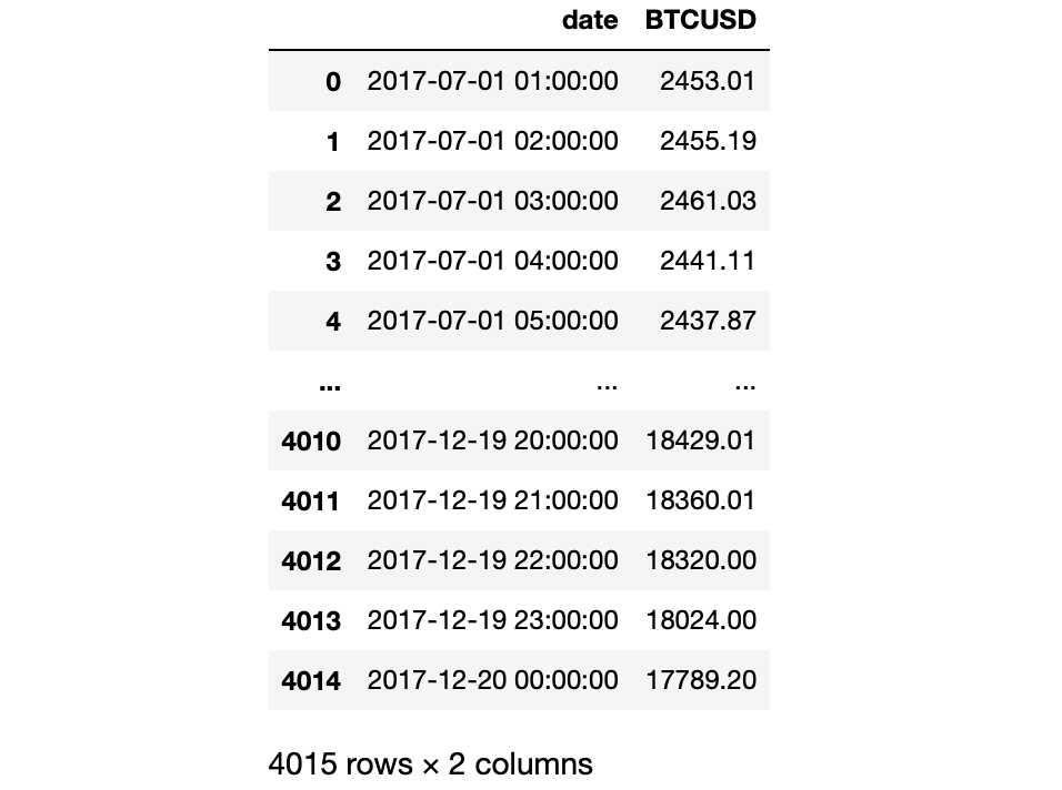
The data is coming from Coinbase crypto-exchange and stored in pandas’ DataFrame as follows:

2. Piecewise Linear Toy Model

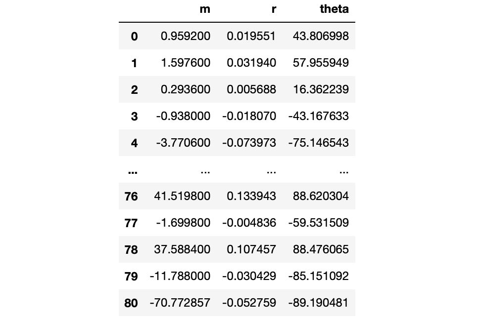
The entire price-series we are going to divide into segments of an equal length. The segments will be non-overlapping. For each one we will fit a linear trend model by fitting a straight line between the first and the last segment’s BTC prices. The line’s slope $m$, the angle of attack $theta$, and the rate of return $r$ per segment will be calculated along the way
$$
m = frac{y_2-y_1}{x_2-x_1}, theta = arctan{m}, r = frac{y_2}{y_1} – 1 ,
$$ respectively. Thanks to them, we will be able to examine a naive relationship between $theta$ and $r$:

# uncomment to run the calculations for 'oos' data
# df = oos.copy()

plt.figure(figsize=(12,6))
plt.plot(df.BTCUSD, color=grey)  # plot Bitcoin time-series
plt.grid()

seglen = 50  # segment lenght (hours)
step = seglen  # vouchsafes non-overlapping
n = df.shape[0]  # number of time-series data points
j = 1

output = list()

# a loop over non-overlapping segments
for i in range(0, n, step):
    x1 = i
    x2 = i + seglen
    if x2 > n: 
        # last segment can be shorter than seglen
        x2 = n - 1
    y1 = df.loc[x1,'BTCUSD']
    y2 = df.loc[x2,'BTCUSD']
    
    # calculations
    slope = (y2-y1)/(x2-x1)  # slope of a linear model
    ror = y2/y1 - 1  # rate of return
    aoa = np.arctan(slope) * 180 / np.pi  # angle of attack
    output.append([slope,ror,aoa])
    
    # updating the plot
    # set a colour code
    if np.mod(j,2) == 0:
        cc = 'r'  # red
    else:
        cc = 'k'  # black
    j += 1
    # plot data segments
    plt.plot([x1, x2], [y1, y2], cc+'-')

plt.xlabel('Number of Hours since  2017-07-01 01:00:00', fontsize=12)    
plt.ylabel('BTC/USD', fontsize=12)
plt.savefig("mer1.png", bbox_inches='tight')
    
# convert Python list into pandas' dataframe object    
output = pd.DataFrame(output, columns=['m', 'r', 'theta'])
o1 = output.copy()
# o2 = outout.copy()

3. Results for 2017 Bull Run

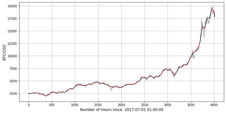
By running the above piece of code, not only we will get the numbers we target to calculate, but also the graphical visualisation of all segments. For clarity, two adjacent segments are marked with different colours:

The output DataFrame stores:

4. Bitcoin 2017 vs 2020 Price Momentum

If we uncomment the line #22 and #68, comment line #67, and rerun the entire code from the beginning, we will generate a new set of results regarding the 2020 Bitcoin bull run dataset. If you, as a homework, frame the code in a form of Python function, you may end up with calling one function for two datasets in two lines of code. No matter as you want to do it, you will be able to compare test sample results (2017) and out-of-sample (2020), for example:

plt.figure(figsize=(9,7))
plt.plot(o1.theta, o1.r, '.', label='2017 BTC bull run')
plt.plot(o2.theta, o2.r, '.', label='2020 BTC bull run')
plt.xlabel('Angle of Attack', fontsize=12)
plt.ylabel('Rate of Return', fontsize=12)
plt.legend(loc=2)
plt.grid()

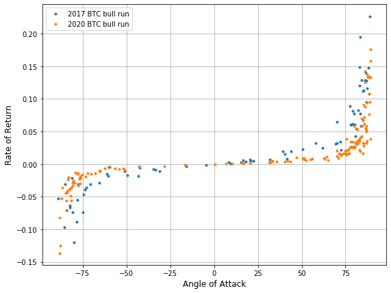
The chart of interest emerges:

In both cases, keeping the model parameters the same, we obtain initial analysis of the relationship in question. By the angle of attack we understand a degree of steepness in the price incline (drop) per segment. The higher the angle the more BTC soars in price per unit of time.

The above results are quite informative. They reveal that both 2017 and 2020 bull runs’ characteristics (in terms of the examined two features) are quite similar. The difference between them is that trading in 2020 appears to be more “bold” or “aggressive” in a sense of the willingness to buy BTC (see $theta gt 75^{circ}$ territory).

The model itself combines the results based on 50 hourly data points (segment length) and depends on a fixed starting points (2017-07-01 01:00:00 and 2020-03-13 01:00:00 for respective bull runs). For the latter, a different selection of the timing may lead to the change of the outputs.

It is rather unlikely to use 2017 results of this model to build a predictive model for 2020 price momentum. The quality of fits and different dynamics in traded cryptocurrency are rather distinct than common. Nonetheless, by checking the same relationship between two similar-but-disjointed bull Bitcoin bull runs, I wanted just to check if there is anything worth further exploration as a cornerstone of my next trading model.

If you have some ideas how this model could be improved, leave your comment. Cheers!

DOWNLOADABLES
btc_bullrun_2017.csv, btc_bullrun_2020.csv

ABOUT THE AUTHOR

Mertcan Coskun is Data Engineer, currently working at International Paper. He received his Bachelor Degree in Industrial Engineering from Marmara University in Istanbul, Turkey in 2016. Mertcan enjoys creating new trading strategies using data driven insights. He continuously learns new things about crypto currencies and signal processing. His LinkedIn profile can be viewed here.