Modelling Slippage for Limit Orders Trading: Adaptive KDE-based Loss Severity Distribution (1)

Placing limit orders for trade execution is both quite popular and handy method in (algo)trading. A trader expects that the executed price of his buy/sell trade will ideally match the one requested in his limit order. Unfortunately, depending on a momentary market/asset liquidity, the difference between both prices can vary or vary significantly. This difference, by many known as an executed slippage, is an undesirable loss due to external factors. It is often a source of frustration because it comes into the game as a hard-to-model free parameter.

There is no closed-form solution for slippage which would work regardless of the market or traded instrument. The estimation of the slippage is often assumed as a constant based on the trader’s judgment and is a subject to modifications in time. The situation gets worse if one trades less liquid assets. Many cryptocurrencies outside the main stream of interest can be a good example here.

We propose a new model for slippage estimation for limit orders applying the concept of the loss severity distribution (LSD). We design the LSD model to be based on Kernel Density Estimation method (KDE) making use of the empirically gathered slippage data from the actual limit-order-based trading. In our model the LSD will represent the probability density function (PDF) of the material losses that a trader may suffer during the execution of the next limit order trade. We propose the 95% Expected Shortfall of LSD as an add-on trade risk charge while a time-dependent modelling of LSD (based on an increasing number of executed trades) provides a trader with a better, quantitative, Bayesian-like risk estimate.

In this Part 1 we begin with a refresher on the empirical estimation of PDF employing ECDFs and histograms. Next, we focus on the use of KDE method as an alternative, discussing its theoretical properties backed by Python examples. In Part 2 we will show how KDE estimation can be viewed as an adaptive method in the estimation of p.d.f. depending on data sample size. We will adopt KDE method for the estimation of LSD using trader’s log of executed limit-order trades for XLM (Stellar cryptocurrency), showing the slippage-free and -affected equity curves. A time-dependent behaviour of 95% quantile of LSD will be postulated as an effective risk charge for individual trades.

1. Estimation of Loss Severity Distribution using KDE Approach

Let $\{x_1, x_2,…,x_n\}$ denote a data sample of size $n$ from a random variable with a PDF of $f$. The goal is to estimate the PDF (or cumulative density function; CDF) given a data set $\{x_i\}^n_{i=1}$.

1.1. ECDF and Histogram Estimates

The distribution of the data points can be visualised and analysed with a help of an (a) Empirical Cumulative Distribution Function (ECDF) or (b) histogram estimate. The alternative is given, inter alia, by the application of KDE approach. The first two methods are considered as quick-and-dirty leaving a room for improvement. In particular, the ECDF is defined as:
\begin{equation}
\hat{F}_n(x=\hat{P} \le x) = \frac{1}{n} \sum_{i=1}^n I_{\{x_i \le x\}}
\end{equation} where
$$
I_{\{x_i \le x\}} =
\begin{cases}
1 & \ \ \ \text{ if} \ \ x_i \le x\\
0 & \ \ \ \text{ otherwise}
\end{cases}
$$ denotes an indicator function. The ECDF assigns equal probabilities of $1/n$ to each value $x_i$ which implies that
\begin{equation}
\hat{P}_n(A) = \frac{1}{n} \sum_{i=1}^n I_{\{x_i \le x\}}
\end{equation} for any set $A$ in the sample space of $X$. On the other hand, if CDF is unknown, we could estimate PDF, $f(x)$, using
$$
\hat{f}(x) = \frac{\hat{F}_n(x+h/2) – \hat{F}_n(x-h/2)}{h} = \frac{ \sum_{i=1}^n I_{\{x_i \in (x-h/2, x+h/2] \}} }{nh}
$$ which uses previous formula with the ECDF in place of the CDF.

More generally, we could estimate $f(x)$ using:
$$
\hat{f}(x) = \frac{ \sum_{i=1}^n I_{\{x_i inI_j\}} }{nh} = \frac{n_j}{nh}
$$ for all $x\in I_j = (c_j – h/2, c_j + h/2]$ where $\{ c_j \}^m_{j=1}$ are chosen constant. This approach to estimating probability density function is know as histogram estimates.

In Python, it can be illustrated in the following way:

import numpy as np
import matplotlib.pyplot as plt

def generate_random_data(n=10):
    rand = np.random.RandomState(2) # fix the randomness state
    return rand.lognormal(mean=0, sigma=1, size=n) # generate random dataset

rdata = generate_random_data(10)

m = 30  # number of bins
hist = plt.hist(rdata, bins=m, density=True)
plt.xlim([0, 6])

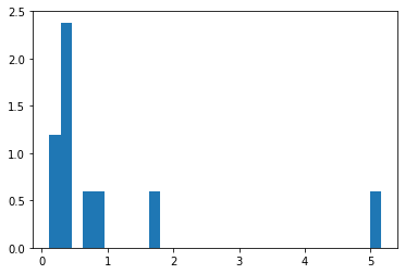where the histogram normalisation has been selected so to make sure that the integral over the entire density is $\int \hat{f}(x) dx = 1$, i.e.

def check_sum(hist):
    density, bins, patches = hist
    widths = bins[1:] - bins[:-1]
    return np.sum((density * widths))

check_sum(hist)  # 1.0

However, different choices for $m$ and $h$ will produce different estimates of $f(x)$. To address this issue, the earliest method that has been proposed here was by Sturges in 1929. I sets $m= \lceil \log_2(n)+1 \rceil$ where $\lceil \cdot \rceil$ denotes a ceiling function. Sturges’ method tends to oversmooth PDF for non-normal data (i.e. it uses too few bins). In 1981 Freedman & Diaconis proposed setting $h = 2(IQR)n^{-1/3}$ where $IQR$ stands for interquartile range, then divide range of data by $h$ to determine $m$.

Histograms are based on the estimation process of a local density. In their case, the points are local to each other if they fall into the same bin. However, the bins are rather an inflexible way of implementing local density estimation. This leads to some undesirable properties, e.g. (a) the resulting estimate is not smooth; (b) an observation may be closer to an observation in the neighbouring bin than it is to the points in its own bin; (c) a selection of bin boundaries can lead to wrongly positioned bin’s density mass. The last case can be illustrated as follows:

bins = np.linspace(0, 2, 30)

fig, ax = plt.subplots(1, 3, figsize=(15, 4),
                       sharex=True, sharey=True,
                       subplot_kw={'xlim':(0, 2),
                                   'ylim':(-0.3, 3.5)})
fig.subplots_adjust(wspace=0.15)
for i, offset in enumerate([0.0, 0.02, 0.1]):
    ax[i].set_title('Offset %.3f' % offset)
    ax[i].hist(rdata, bins=bins + offset, density=True) # plot histogram
    ax[i].plot(rdata, np.full_like(rdata, -0.15), '|k',
               markeredgewidth=1)  # mark individual data points

where a small offset applied to bin’s position changes the resulting densities in respect to the actual data points.

These properties make a justification for the application of methods taking weighted local density estimates at each observation $x_i$ and then aggregating them to yield an overall density. For example, one may consider estimation of the density at the point $x_0$ by taking the local density of the points within certain distance $h$ about $x_0$, i.e.
$$
\hat{f}(x_0) = \frac{ n^{-1} \sum_{i=1}^n I_{ \{ |x_i – x_0| \le h \}} }{2h} \ .
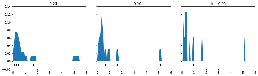
$$ This solves one problem of the histogram, namely, it ensures that no point further away from $x_0$ than $x_i$ will contribute more than $x_i$ does to the density estimate. Unfortunately, the resulting density estimate remains bumpy due to a limiting value of $h$. A good illustration of this process is the following code:

fig, ax = plt.subplots(1, 3, figsize=(15, 4),
                       sharex=True, sharey=True,
                       subplot_kw={'xlim':(0, 6),
                                   'ylim':(-0.02, 0.14)})

fig.subplots_adjust(wspace=0.15)
for i, h in enumerate([0.25, 0.1, 0.05]):
    x_d = np.linspace(0, 6, 100)
    density = sum((abs(xi - x_d) < h) for xi in rdata)
    density = density / density.sum()
    ax[i].set_title('h = %.2f' % h)
    ax[i].fill_between(x_d, density)
    ax[i].plot(rdata, np.full_like(x, -0.01), '|k', markeredgewidth=1)

where three different limiting values of $h$ are considered, leading to different density estimates:

1.2. Kernel Density Estimation (KDE)

Instead of giving every point in the neighbourhood equal weight, one may assign a weight which dies off towards zero in a continuous fashion as one gets further away from the target point $x_0$.

Consider estimators of the following form:
$$
\hat{f}_h(x_0) = \frac{1}{nh} \sum_{i=1}^n K\left( \frac{x_i – x_0}{h} \right)
$$ where $h$, which controls the size of the neighbourhood around $x_0$, is a smoothing parameter or a bandwidth. The function $K$ is called the kernel. It controls the weight given to the observation $\{x_i\}$.

Given all above, the kernel function $K$ must satisfy three properties, namely: (1) $\int K(u)du = 1$; (2) be symmetric around zero, i.e. $\int uK(u) du = 0$; and (3) $\int u^2K(u)du = \mu_2(K) > 0$. A popular choice of $K$ is the Gaussian kernel function defined as:
$$
K(u) = \frac{1}{\sqrt{2\pi}} \exp \left( -\frac{u^2}{2} \right)
$$ with the only shortcoming that its support runs over the entire real line. Occasionally it is desirable that a kernel have a compact support. In such cases one may use e.g. the Epanechnikov or tri-cube compact kernels. For the needs of this articles, we will skip their application.

For a fixed $h$s, the kernel density estimations are not consistent. However, if the bandwidth decreases with a sample size at an appropriate rate, then they are consistent, regardless of which kernel is used. It quickly became clear that the value of the bandwidth is of critical importance, while the shape of $K$ has little practical impact!

Assuming that the underlying density is sufficiently smooth and that the kernel function has a finite 4th moment, it has been shown, e.g. by Wang & Jones in 1995 that by the use of Taylor series one can get the following estimations of bias and variance:
$$
\text{Bias}\{\hat{f}_h(x)\} = \frac{h^2}{2} \mu_2(K) f”(x) + o(h^2)
$$
$$
\text{Var}\{\hat{f}_h(x)\} = \frac{1}{nh} \int K^2(u)du f(x) + o\left( \frac{1}{nh} \right)
$$ In practice, we wish to find the best estimate, $\hat{f}_h(x)$, of the true PDF $f(x)$ for our data sample. The Mean Integrated Squared Error (MISE) is a widely used choice of an overall measure of the discrepancy between $\hat{f}_h(x)$ and $f(x)$, defined as:
$$
\text{MISE}(\hat{f}_h) = E \left\{ \int [f(y)-\hat{f}_h(y)]^2 dy \right\} = \int \text{Bias}(\hat{f}_h(y))^2 dy + \int \text{Var}(\hat{f}_h(y))dy
$$ or, in general, as:
$$
\text{MISE}(\hat{f}_h) = E \left\{ \int f(y)^2 dy \right\} – 2E \left\{ \int f(y)\hat{f}_h(y)dy dy \right\} + E \left\{ \int \hat{f}_h^2(y)dy dy \right\} \ .
$$ In order to minimise the MISE, one aims to minimise:
$$
E \left\{ \int f(y)^2 dy \right\} – 2E \left\{ \int f(y)\hat{f}_h(y)dy dy \right\} \ \ \ \ \ \ \ \ \ \ \text{(*)}
$$ expression with respect to the bandwidth $h$. An unbiased estimate of the first term of $\text{(*)}$ given by
$$
\int f(y)^2dy
$$ is usually evaluated using numerical integration techniques. As it comes to the second term of $\text{(*)}$, it was shown by Rudemo in 1982 and Bowman in 1984 that an unbiased estimate of it is:
$$
-\frac{2}{n}\sum_{i=1}^n \hat{f}_h^{(i)} (x_i)
$$ where
$$
\hat{f}_h^{(i)} (x_i) = \frac{1}{h(n-1)} \sum_{j\ne i} K \left( \frac{x-x_j}{h} \right)
$$ is leave-one-out estimate of $\hat{f}_h$ and the entire method is know as Least Squares Cross-Validation (LSCV) approach to determine the most optimal bandwidth $h$. In Python, we can get such estimation in the following way:

from sklearn.neighbors import KernelDensity
from sklearn.model_selection import GridSearchCV, LeaveOneOut

# Step 1. 
# Fit the KDE model to rdata
#
bw = 1.0  # default value
kde = KernelDensity(bandwidth=bw, kernel='gaussian')
kde.fit(rdata[:, None])

# score_samples returns the log of the probability density
x_d = np.linspace(0, 6, 1000)
logprob = kde.score_samples(x_d[:, None])
density = np.exp(logprob)
density = density / density.sum() # normalise density

plt.figure(figsize=(12,5))
plt.fill_between(x_d, density, alpha=0.5, label='Bandwidth = %.5f' % bw)
plt.plot(x, np.full_like(x, -0.0001), '|k', markeredgewidth=1)
plt.xlim([0, 6])


# Step 2.
# Find the optimal bandwidth values
#
bandwidths = 10 ** np.linspace(-1, 1, 1000)
grid = GridSearchCV(KernelDensity(kernel='gaussian'),
                    {'bandwidth': bandwidths},
                    cv=LeaveOneOut())
grid.fit(rdata[:, None]);
bw = grid.best_params_['bandwidth']


# Step 3.
# Re-fit the KDE model to rdata with the optimal bandwidth
#
kde = KernelDensity(bandwidth=bw, kernel='gaussian')
kde.fit(rdata[:, None])
logprob = kde.score_samples(x_d[:, None])
density = np.exp(logprob)
density = density / density.sum() # normalise density

plt.fill_between(x_d, density, alpha=0.5, label='Bandwidth = %.5f (optimal)' % bw)
plt.plot(x, np.full_like(x, -0.0001), '|k', markeredgewidth=1, label='Data Points')
plt.xlim([0, 6])
plt.legend(loc=1)

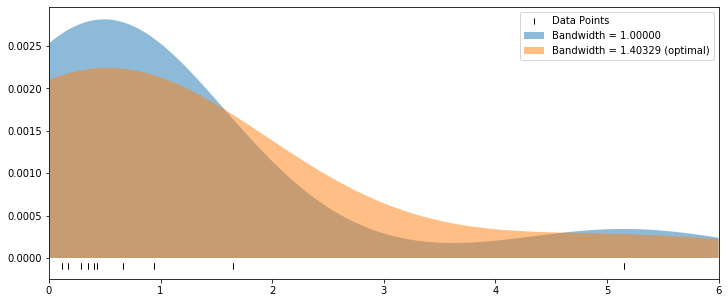
where we employ the Gaussian kernel with a default bandwidth equal 1 as a starting point.

The data are fitted making use of such selected setup of KDE and result plotted in light blue colour in the chart. Next, the grid search (cross-validation) is run to determine the most optimal bandwidth for the data set. It turns out its value is higher than default and equal 1.403. Lastly, the data are re-fitted with the optimal bandwidth value to determine the most optimal fit of KDE to the data (note that their number is $n=10$ in this example). A new density plot is added in light orange colour for comparison:

The LSCV is also referred to as the unbiased cross-validation since
$$
E[\text{LSCV}(h)] = E \left\{ \int [f(y)-\hat{f}_h(y)]^2 dy \right\} – \int f(y)^2dy = \text{MISE} \ – \int f(y)^2dy
$$
The LSCV, as one may think, is not the only method that has been developed and proposed in order to find the most optimal bandwidth $h$. For instance, Silverman (1986) postulated a Rule of Thumb; Scott & Terrel (1987) described Biased Cross-Validation; Sheather & Jones (1991), Jones, Marron, & Sheather (1996) proposed Plug-in Methods; the Local Likelihood Density Estimates were suggested by Hjort & Jones (1996) and Loader (1996) followed by Data Sharpening approach of Hall & Minnotte in 2002. A concise overview of a theory and guidance on the application of all these methods one can find in Sheather (2004) who summarises, inter alia, that Sheather-Jones plug-in bandwidth is widely recommended due its overall good performance. However, for hard to estimate densities, i.e. these for which $|f”(x)|$ varies widely, it tends to oversmooth. In these situations, the LSCV often provides protection against this undesirable feature due to its tendency to undersmooth.