Previously, in Part 1, we described the method using websockets to “listen” to the most recent update of coin prices as broadcast by Binance exchange. We developed Python code around that and showed how to capture and record OHLC prices for an individual coin. The information was coming from so-called kline object which represented a candlestick price formation for a defined duration of 1 minute. The visualisation of all interim prices, i.e. broadcast between candlestick’s opening and closing times, we addressed separately in Part 2.
Binance’s API also offers a method to request most recent prices for a whole list of coins we are interested in. This method has been described in the API’s documentation here. Alternatively, the same data can be fetched in a similar manner using CryptoCompare’s API as provided here.
Regardless of the method we choose, we are going to face a very common problem in data engineering regarding the fact that transmitted and recorded (e.g. in .csv format) prices for a larger number of coins (N-Asset Portfolio) will never arrive precisely at the times we wish them to be, i.e. they will be asynchronously captured. If our code aims to grab the prices for 100 coins every 5 seconds, there is a very low probability that the arrival times will be aligned and useful for any further quantitative analysis (e.g. examining linear correlation on 5-second timescales) which requires aligned data points.
In today’s article, we will show how such alignment of prices can be done given recorded prices of 100 coins on 5 second intervals.
1. Data
Let’s say as the output of our code responsible for grabbing most recent prices (called in a loop every five seconds) we gather a collection of .csv files with prices of ca. 100 coins given as a sorted list according to the current Coin Market Cap:
import os
from pathlib import Path
import glob
from datetime import datetime
import pandas as pd
import numpy as np
from matplotlib import pyplot as plt

# data
data_folder = './data_5s/'
fnames = list()
for file in glob.glob(data_folder + 'coin_prices_live*'):
    fnames.append(file)

fnames = sorted(fnames)

# first 10 file names
print(fnames[0:10])
['./data_5s/coin_prices_live_20220518213700.csv',
 './data_5s/coin_prices_live_20220518213706.csv',
 './data_5s/coin_prices_live_20220518213712.csv',
 './data_5s/coin_prices_live_20220518213717.csv',
 './data_5s/coin_prices_live_20220518213723.csv',
 './data_5s/coin_prices_live_20220518213729.csv',
 './data_5s/coin_prices_live_20220518213735.csv',
 './data_5s/coin_prices_live_20220518213740.csv',
 './data_5s/coin_prices_live_20220518213746.csv',
 './data_5s/coin_prices_live_20220518213752.csv']
# last 5 file names
print(fnames[-5:])
['./data_5s/coin_prices_live_20220519112435.csv',
 './data_5s/coin_prices_live_20220519112441.csv',
 './data_5s/coin_prices_live_20220519112447.csv',
 './data_5s/coin_prices_live_20220519112452.csv',
 './data_5s/coin_prices_live_20220519112458.csv']
In other words, data recording started exactly on 2022-05-18 21:37:00 UT+2 and ended on 2022-05-19 11:24:58 UT+2, covering nearly 14 hours. The file names contain the timestamp when the data request was sent and were supposed to be sent out every 5 seconds. However, as one can easily notices, the differences between various consecutive timestamps fall between 5 up to even 7 seconds. This is caused the the fact of technical delays in data processing.
The second important aspect here is that by executing such procedure for data recording, we make a silent assumption that “recorded time” corresponds to the most recent value of coin(s) prices regardless the time the price has been updated in the database of the data provider. The latter can be read from the files themselves, e.g.:
pd.read_csv('./data_5s/coin_prices_live_20220518213700.csv')

The first column contains the timestamps with the last price update. One can notice that it is earlier than 21:37:00 UT+2. However, we assume the corresponding prices are the best known prices when fetched at 21:37:00 UT+2 we can work with.
Given the data files, we merge all necessary information into a single DataFrame, e.g.:
fi = True
for fname in fnames:  #_set:
    recorded_at = datetime.strftime(datetime.strptime(fname[-18:-4],'%Y%m%d%H%M%S'),
                                    '%Y-%m-%d %H:%M:%S')
    tmp = pd.read_csv(fname)
    tmp['RECORDED_AT'] = pd.to_datetime(recorded_at)
    tmp = tmp[['RECORDED_AT', 'FROMSYMBOL', 'PRICE']]
    if fi:
        df = tmp.copy()
        del tmp
        fi = False
    else:
        df = pd.concat([df, tmp])
        del tmp

print(df)
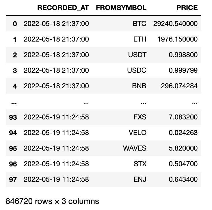
where we have collected prices of 98 coins:
coin_list = df.FROMSYMBOL.unique().tolist()
print(coin_list, len(coin_list))
['BTC', 'ETH', 'USDT', 'USDC', 'BNB', 'XRP', 'SOL', 'BUSD', 'ADA', 'AVAX', 'DOT', 'DOGE',
 'FTT', 'GMT', 'WBTC', 'APE', 'TRX', 'LINK', 'SHIB', 'XLM', 'MATIC', 'DAI', 'AXS', 'CRO',
 'UNI', 'LTC', 'LEO', 'KLAY', 'NEAR', 'ICP', 'BCH', 'SAND', 'ALGO', 'OKB', 'FLOW', 'ATOM',
 'GALA', 'XMR', 'VET', 'QNT', 'DFI', 'MANA', 'EGLD', 'CRV', 'DYDX', 'GNO', 'HBAR', 'KCS',
 'ILV', 'GRT', 'IMX', 'XDC', 'FIL', 'XTZ', 'RUNE', 'PCI', 'HT', 'MKR', 'LDO', '1INCH',
 'EOS', 'AAVE', 'AMP', 'NEXO', 'CELO', 'CAKE', 'ZEC', 'THETA', 'LUNA', 'UST', 'ENS',
 'CHZ', 'XRD', 'RLY', 'NEO', 'CVX', 'BSV', 'MIOTA', 'MC', 'HNT', 'AR', 'XCH', 'USDP',
 'MINA', 'QTF', 'FTM', 'GT', 'XEC', 'USDN', 'TUSD', 'ZIL', 'ROSE', 'KSM', 'FXS', 'VELO',
 'WAVES', 'STX', 'ENJ'] 98
2. 5-Second Price-Series Alignment Procedure for N-Asset Portfolio
The easiest way here is to convert the above DataFrame into a new one, with columns representing the prices of coins (expressed in USD) sampled every 5 seconds. Due to a large number of coins, gaps in the data may occur. The procedure is as following. First, we create a template DataFrame with a time index spanned beween:
# template
ts, te = df.RECORDED_AT.min(), df.RECORDED_AT.max()
print(ts, te)
Timestamp('2022-05-18 21:37:00'), Timestamp('2022-05-19 11:24:58')
i.e.
resample_index = pd.date_range(start=ts, end=te, freq='5S')
print(resample_index)
DatetimeIndex(['2022-05-18 21:37:00', '2022-05-18 21:37:05',
               '2022-05-18 21:37:10', '2022-05-18 21:37:15',
               '2022-05-18 21:37:20', '2022-05-18 21:37:25',
               '2022-05-18 21:37:30', '2022-05-18 21:37:35',
               '2022-05-18 21:37:40', '2022-05-18 21:37:45',
               ...
               '2022-05-19 11:24:10', '2022-05-19 11:24:15',
               '2022-05-19 11:24:20', '2022-05-19 11:24:25',
               '2022-05-19 11:24:30', '2022-05-19 11:24:35',
               '2022-05-19 11:24:40', '2022-05-19 11:24:45',
               '2022-05-19 11:24:50', '2022-05-19 11:24:55'],
              dtype='datetime64[ns]', length=9936, freq='5S')
followed by
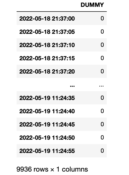
template = pd.DataFrame(0, index=resample_index, columns=['DUMMY'])
print(template)
In the next step, in the loop over all coins, we resample coin’s price-series with 5 second resolution applying securely the averaging of the price records falling into the same 5 second bin (line #55). Though this is very unlikely to happen, this step is applied for consistency:
fi = True
for coin in coin_list:
    tmp = df[df['FROMSYMBOL'] == coin]
    tmp = pd.DataFrame(tmp.resample('5S', on='RECORDED_AT').PRICE.mean())
    tmp.rename(columns={'PRICE' : coin}, inplace=True)
    tmp.index = pd.to_datetime(tmp.index)
    if fi:
        ts = pd.merge(left=template, right=tmp, how='left', left_index=True,
                      right_index=True)
        fi = False
    else:
        ts = pd.merge(left=ts, right=tmp, how='left', left_index=True,
                      right_index=True)

del ts['DUMMY']  # get rid of this column

print(ts)
In lines #59 and #63 we apply LEFT JOIN operation on the resampled series starting from merging the template DataFrame with BTC price-series, and next adding up the series for ETH, USDT, USDC, BNB, XRP, SOL, etc. The output DataFrame takes its final shape:
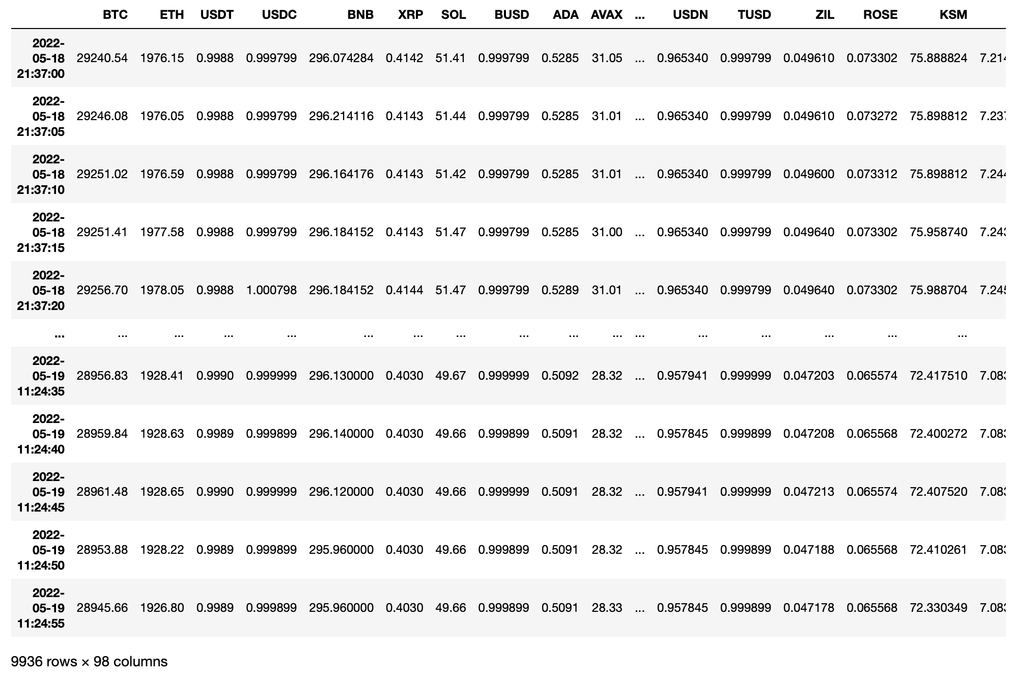
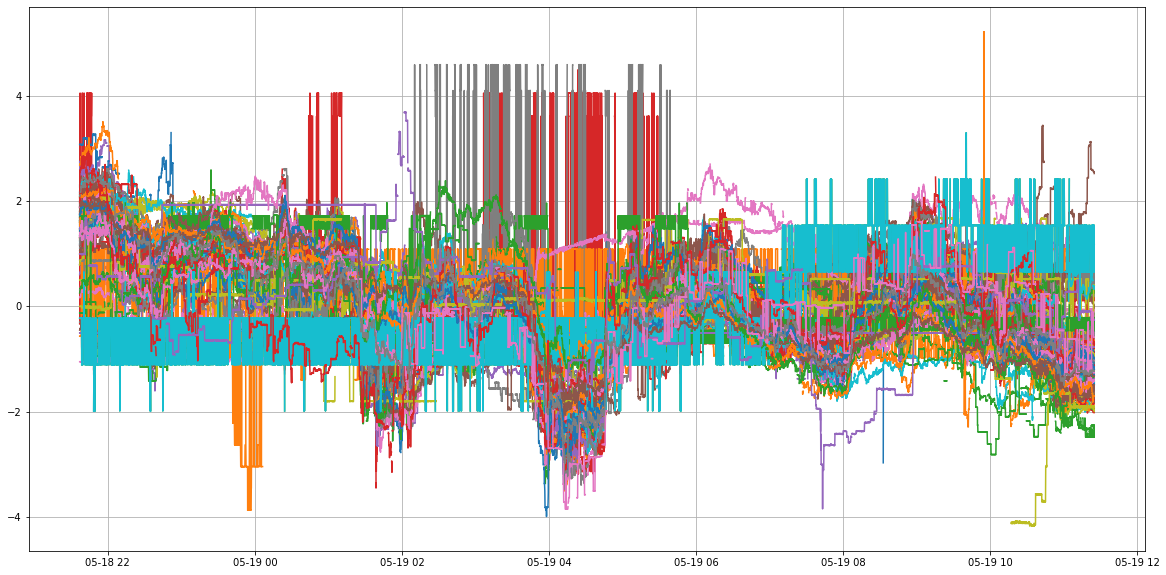
possible to visualise by plotting normalised price-series of all 98 coins:
plt.figure(figsize=(20,10))
plt.plot((ts - ts.mean()) / ts.std(ddof=1))
_ = plt.grid()
In the forthcoming Part 4 we will dive into the analysis of N-asset crypto-portfolio covering distance correlation measure vs Pearson’s standard approach.
Explore Further
→ Hacking 1-Minute Cryptocurrency Candlesticks: (1) Capturing Binance Exchange Live Data Stream
→ Hacking 1-Minute Cryptocurrency Candlesticks: (2) Custom Candlestick Charts in Plotly
→ XRP-based Crypto Investment Portfolio Inspired by Ripple vs SEC Lawsuit
→ How to Design Intraday Cryptocurrency Trading Model using Bitcoin-based Signals?