There is a huge number of ways how one can transform financial times-series in order to discover new information about changing price dynamics. We talk here about certain transformation that takes price time-series (or return-series) and transforms it into a new domain. Every solid textbook on Time-Series Analysis lists ample examples. In this article we are going to describe in greater detail of the Matching Pursuit algorithm, a natural method taking its roots from both Fourier transform and Continuous Wavelet Transform. Keep reading to learn more!
1. Fourier Transform
Interestingly, there is little to few information on the usefulness of Fourier Transform (FT) applied to financial time-series. No wonder why. In discrete edition of the FT, the incoming time-series, $x(t)$ where $t$ denotes time, is transformed into frequency domin of information, $P(f)$ where $f$ is frequency and $P$ represents effective power of transformed signal, e.g.
$$
P(f_j) = \left| \sum_{l=0}^{N-1} (x(t_l) – \bar{x}) e^{-i2\pi jl/N} \right|^2
$$ where $\bar{x}$ denotes mean values and $N$ number of data points in $x(t)$ and $f_j$ is frequency index. The quantity of $P(f)$, defined above, often is referred to as Fourier Power Spectrum. The key information here is what it does. In plain English, the FT scans a wide range of frequencies and matches a degree of similarity between a sine wave of frequency $f_j$ and the signal $x(t_l)$ itself. If such “correlation” exists, the $P$ (or the inner product between the signal and base sine function) will deliver a large value compared to the other frequencies.
In other words, FT is best if we look for purely periodic oscillations in our time-series. The best scenario would be if such periodic pattern is active along the entire record of the examined signal; it loses it power if it lasts shorter under additional condition, i.e. if signal-to-noise ratio allows for its detection. Signal that is a realisation of white noise has a flat power spectrum while time-series with long up/down-trends will reveal lots of colour noise in low frequency section. In a log-log representation of $P(f)$, such colour noise is modelled by a power-law model, $P(f) \propto f^{-\alpha}$ where the higher $\alpha$ the steeper slope or stronger trend in time-domain of the signal.
In real life applications of FT, very rarely trading signals are dominated by distinct periodicities. Due to unlimited market factors, the power spectrum may display broader “peaks”, suggesting the existence of a latent dumping process or $x(t) \propto \sin(2\pi f_0 t)\exp(-t/\tau)$ where $\tau$ denotes a damping time-scale. In science, we talk about not periodic but a bunch of periodic or localised periodic or quasi-periodic oscillations (QPOs) present in the signal. A Lorentzian has
$$
P(f)= A \Delta f/[(f-f_0)^2 +(\Delta f/2)^2]
$$ defined by a centroid frequency, $f_0$, a full width at half maximum (FWHM) of $\Delta f$ and amplitude. A ratio of the QPO frequency to Lorentzian FWHM is known as a quality factor, $Q=f_0/\Delta f$. The distinguishing feature of the QPO as opposed to the noise components is that its quality factor can be large. The higher $Q$ the wider QPO. All these parameters are correlated in the low-frequency QPO, with the amplitude and quality factor increasing along with the increase in centroid frequency.
It is obviously important to know what sets the (lack of) coherence of the QPO. Are QPOs composed of a set of longer-lasting continuous modulations or are they rather fragmented in time with frequencies concentrated around the peak QPO frequency? Is there any correlation between observed oscillations or they are preferably excited in a random manner? To answer these questions we need to resolve and understand the internal structure of detected QPOs i.e. to study the behaviour of the QPO on timescales which are short compared to its observed broadening. A continuous modulation would then show up as a continuous drift in QPO frequency with time, while a series of short timescale oscillations will show up as disjoint sections where the QPO is on and off.
One way to do this is using dynamical power spectra (spectrograms; hereafter also referred to as Short-Fourier Transform or STFT for simplicity). While the actual techniques for this can be quite sophisticated in essence, an observation of length $T$ sampled every $\Delta t$ (giving a single power spectrum spanning frequencies $1/T$ to $1/(2\Delta t)$ in steps of $1/T$) is spilt into $N$ segments of length $T/N$. This gives $N$ independent power spectra spanning frequencies $N/T$ to $1/(2\Delta t)$ but crucially, the resolution is now lower, at $N/T$. While this is useful in tracing the evolution of the QPO, it introduces “instrumental” frequency broadening from the windowing of the data which prevents us following the detailed behaviour of the QPO on the required timescales.
The real problem with such Fourier analysis techniques is that they decompose the signal onto a basis set of sinusoid functions. These have frequency $f$, with resolution $\Delta f=N/T$, but exist everywhere in time across the duration of the observation $t_{dur}=T/N$. In the same way that the Heisenberg uncertainty principle sets a limit to the measurement of momentum and location of a particle, namely $\Delta p_x \Delta x \geq h/2\pi$ where $h$ is a Planck constant, there is a Heisenberg-Gabor uncertainty principle setting the limiting frequency resolution for time-series analysis. This states that we cannot determine both the frequency and time location of a power spectral feature with infinite accuracy.
2. Wavelet Transform
Instead, if the QPO is really a short-lived signal, we will gain in resolution and get closer to the theoretical limit by using a set of basis functions which match the underlying physical shape of the QPO. This is the idea behind wavelet analysis. For example, one particular basis function shape is the Morlet wavelet, which is a sinusoid of frequency $f$, modulated in amplitude by a gaussian envelope such that it lasts only for a duration $t_{dur}$. The product $f \times t_{dur}$ is set at a constant, fixing the number of cycles seen in the basis function. The lightcurve is then decomposed on these basis functions, calculated over a set of frequencies so that the basis function shape is maintained (i.e. that the oscillation consists of 4 cycles, so low frequencies have longer $t_{dur}$ than high frequencies). The resolution adjusts with the frequency, making this a more sensitive technique to follow short duration signals.
However, the problem is that the basis functions chosen in wavelet analysis may not be appropriate. For example, we assumed above that these functions have a fixed shape, lasting for a fixed number of oscillations at all frequencies. In practice, this may not be the best description of the QPO. Perhaps the QPO is made from a set of signals which have a distribution of durations, where $f\times t_{dur}$ is not constant. We will maximise the resolution with which we can look at the QPO if and only if we use basis functions which best match its
shape.
To do this one can propose the application of the Matching Pursuit algorithm (MP). This is an iterative method for signal decomposition which aims at retrieving the maximum possible theoretical resolution by deriving the basis functions from the signal itself. We specifically use this as an extension of the wavelet technique by setting the MP basis functions as Gaussian amplitude modulated sinusoids as before, but allowing the product $f\times t_{dur}$ to be a free parameter (a.k.a. Gabor atoms).
3. Matching Pursuit algorithm
Signal time-frequency analysis can be compared to speaking in a foreign language. In each language we use words. Words are needed to express our thoughts, problems, ideas, etc. By a smart selection of proper words we can say and explain whatever we wish. A whole collection of words can be gathered in the form of a dictionary. One can express simple thoughts using a very limited set of words from a huge dictionary (a subset). The same can be applied to a time-series analysis. In order to describe the signal one needs to use a minimum available set of functions $-$ orthonormal basis functions.
Description of the signal $x_n$ which uses only basis functions $g_n \ (n=1,…,N’)$ is therefore limited. This is often the case with wavelet transform. In order to improve signal description, one can increase the size of a basic dictionary by adding extra functions. Such a dictionary’s enlargement introduces a redundancy what is a natural property of all, for instance, foreign languages. The most reliable signal description can be achieved by a signal approximation
$$
x \approx \sum_{n=1}^{M\lt N’} a_{\gamma,n} g_{\gamma,n}
$$ where coefficients $a_{\gamma,n}$ are defined simply as the inner products of basis functions $g_{\gamma,n}$ with a signal:
$$
\langle x, g_{\gamma,n} \rangle = \int_{-\infty}^\infty x(t) g_{\gamma}(t) dt
\approx \sum_{n=1}^{M\lt N’} x_n g_{\gamma,n}
$$ and $\gamma$ refers to a set of parameters of function $g$.
In each approximation, a relatively small number of functions is generally required. For each case the signal is projected onto a set of basis functions, therefore, in other words, its representation is always fixed. However, what if one may approach the signal decomposition problem from the other side, i.e. to fit the singal representation to the signal itself? One can achieve it by choosing from a huge dictionary of pre-defined functions a subset of functions which would best represent the signal. Such solution had been proposed by Mallat & Zhang (1993) and is known under the name of Matching Pursuit algorithm.
3.1. Algorithm
Matching Pursuit (MP) is an iterative procedure which allows to choose from a given, redundant dictionary $D$, where $D=\{ g_1, g_2,…,g_n\}$ such that $||g_i||\!=\!1$, a set of $m$ functions $\{ g_i \}_{m\lt n}$ which match the signal as well as possible. $D$ is defined as a family (not a basis) of time-frequency waveforms that can be obtained by time-shifting, scaling and, what is new comparing to wavelet transform, modulating of a single even function $g\in L^2(\Re)$; $\Vert g \Vert=1$;
$$
g_\gamma = \frac{1}{\sqrt{a}} g\left(\frac{t-b}{a}\right) e^{i f t}
$$
where an index $\gamma$ refers to a set of parameters:
$$
\gamma=\{ a,b,f \} .
$$ Each element of the dictionary is called an atom and usually is defined by a Gabor function, i.e. a Gaussian function modulated by a cosine of frequency $f$:
$$
g_\gamma(t)\!=\!K_\gamma(t) G_\gamma(t)\! =\!
K_\gamma(t)
\exp\left[-\pi\left(\frac{t-b}{a}\right)^2\right]
\cos\left( 2\pi ft + \phi \right)
$$ where
$$
K_\gamma(t) = \left( {\sum_{t=-\infty}^\infty G_\gamma(t)^2} \right)^{-1/2}
$$ and $a$ denotes the atom’s scale (duration; in this paper also referred to as atom’s life-time} and $b$ — time position. A selection of Gabor functions for purposes of MP method is fairly done as they provide optimal joint time-frequency localisation.
In the first step of MP algorithm, a function $g_{\gamma,1}$ is chosen from $D$ which matches the signal $x$ best. In practice it simply means that a whole dictionary $D$ is scanned for such $g_{\gamma,1}$ for which a scalar product $|\langle x,g_{\gamma,1}\rangle|\in\Re$ is as large as possible. Therefore, a signal can be decomposed into:
$$
x = \langle x,g_{\gamma,1}\rangle g_{\gamma,1} + R^1x
$$ where a $R^1x$, a residual signal, has been denoted. In the next step, instead of $x$, the remaining signal $R^1x$ is decomposed by finding a new function, $g_{\gamma,2}$, which matches $R^1x$ best. Such consecutive steps can be repeated $p$ times where $p$ is a given, maximum number of iterations for signal decomposition. In short, MP procedure can be denoted as:
$$
\left\{ \begin{array}{l}
R^0x = x\\
R^ix = \langle R^ix,g_{\gamma,i}\rangle g_{\gamma,i} +
R^{i+1}x \\
g_{\gamma,i} = \arg\max_{g_{\gamma,i’}\in D}
|\langle R^ix,g_{\gamma,i’}\rangle| .
\end{array}
\right.
$$
Davis et al. (1994) showed that for $x\in H$ the residual term $R^ix$ defined by the induction equation above satisfies:
$$
\lim_{i\rightarrow +\infty} \Vert R^ix\Vert = 0
$$ i.e., when $H$ is of finite dimension, $\Vert R^ix\Vert$ decays to zero. Hence, for a complete dictionary $D$, the Matching Pursuit procedure converge to $x$:
$$
x = \sum_{i=0}^\infty \langle R^ix,g_{\gamma,i}\rangle g_{\gamma,i}
$$ where orthogonality of $R^{i+1}x$ and $g_{\gamma,i}$ in each step implies energy conservation:
$$
\begin{array}{ll}
\Vert x \Vert^2\! & =
\sum_{i=0}^{p-1}
|\langle R^ix,g_{\gamma,i}\rangle|^2
+ \Vert R^px\Vert^2 \\
& = \sum_{i=0}^{\infty}
|\langle
R^ix,g_{\gamma,i}\rangle|^2 \ .
\end{array}
$$
3.2. Time-frequency representation
From abovementioned formula one can derive a time-frequency distribution of signal’s energy by adding a Wigner-Ville distribution of selected atoms $g_\gamma$:
$$
\begin{array}{ll}
(Wx)(t,f) & = \sum_{i=0}^\infty |\langle R^ix,g_{\gamma,i}\rangle|^2
(Wg_{\gamma,i})(t,f) + \\
& \sum_{i=0}^\infty \sum_{j=0,j\ne i}^\infty
\langle R^ix,g_{\gamma,i}\rangle
\langle R^jx,g_{\gamma,j}\rangle^\ast \ \ \times \\ \nonumber
& \ \ \ \ \ \ \ \ \ \ \ \ \ \ \ \ \ \ \ \ \
\ \ \ \ \ \ \ \ \ \ \ \ \ \ \ \times \ \
(W[g_{\gamma,i},g_{\gamma,j}])(t,f)
\end{array}
$$ The double sum present in the above equation corresponds to cross-terms present in the Wigner-Ville distribution. In MP approach, one allows to remove these terms directly in order to obtain a clear picture of signal energy distribution in the time-frequency plane $(t,f)$. Thanks to that, {\it energy density} of $x$ can be defined as follows:
$$
(Ex)(t,f) = \sum_{i=0}^\infty
|\langle R^ix,g_{\gamma,i}\rangle|^2
(Wg_{\gamma,i})(t,f) .
$$
Since Wigner-Ville distribution of a single time-frequency atom $g_\gamma$ satisfies:
$$
\int_{-\infty}^{\infty} \int_{-\infty}^{\infty}
(Wg_{\gamma,i})(t,f) dt df = \Vert g_\gamma \Vert^2 = 1
$$ thus combining the above with energy conservation of the MP expansion yields:
$$
\int_{-\infty}^{\infty} \int_{-\infty}^{\infty}
(Ex)(t,f) dt df = \Vert x \Vert^2
$$
what justifies interpretation of $(Ex)(t,f)$ as the energy density of signal $x$ in the time-frequency plane.
3.3. Stochastic Dictionaries
In practical computation of MP algorithm, sampling of a discrete signal of length $N=2^L$ is governed by an additional parameter $j$: an octave (Mallat \& Zhang 1993). The scale $a$ corresponding to an atom’s scale is derived from a dyadic sequence of $a=2^j, 0\le j\le L$. Thus, parameters $b$ and $f$, corresponding to atom’s position in time and frequency, respectively. By resolution in the MP one may understand the distance between centres of atoms neighboring in time or in frequency. A dyadic sampling pattern proposed by Mallat & Zhang has been found to suffer from a statistical bias introduced in the atom parametrisation. Durka et al. (2001) proposed a solution to this problem by application of stochastic dictionaries. In this approach the parameters of dictionary’s waveforms are randomised before each decomposition by drawing their values from continuous ranges.
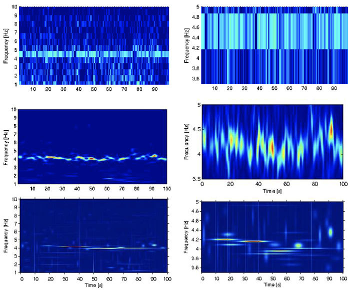
Figure. Time-frequency analysis performed for an exemplary signal: (upper) STFT calculated for the first 100 s long data segment revealing QPO activity around a central frequency of 4 Hz (46 point sliding window); (middle) the corresponding wavelet power spectrum derived with a Morlet analysing function; (bottom) Matching Pursuit decomposition (based on 3 × 10⁶ atom dictionary) displayed as energy density $(E x)(t, f )$
3.4. Number of MP Decompositions for a Single Signal
Durka et al. (2001) pointed at a significant aspect of Matching Pursuit method: an ability to represent signals with continuously changing frequency. In the standard approach one aims at calculation of a single MP decomposition for a given signal using a large redundant dictionary of pre-defined functions (e.g. $3\times 10^6$ atoms). When the signal contains continuously changing frequency in time a single MP decomposition will provide energy density plot to be composed of a number of single Gabor atoms. Therefore, such a view remains far different from expectations.
On the way of experiments Durka et al. (2001) discovered that by introduction of stochastic dictionaries and averaging a larger number, say 100, of the MP energy density plots together one can uncover continuously changing signal frequency. The trick is to use for every MP decomposition performed for the same signal a new stochastic dictionary and of much smaller size, e.g. composed of $5\times 10^4$ atoms only.
It is wise to check whether for all data segments you analyse the MP results are insensitive to the way of MP computation, i.e. irrespective of the dictionary size used and the application of aforementioned MP map averaging process. In this way, we are able to exclude a scenario in which QPOs are being generated due to long timescale oscillations of continuously changing frequency.
References
Durka, P, 2001, Matching Pursuit and Unification in EEG Analysis (Engineering in Medicine & Biology) 1st Ed.
Jump Deeper
Structure Function: Forgotten Detection Tool for Periodic Signals in Non-Stationary Processes
Modern Time Analysis of Black Swans