The Longest Winning Bitcoin Strategy

What is the best winning Bitcoin strategy? A tough one! However, one can verify some numbers leading to interesting results.

In the previous article Estimating Probability of Bitcoin Pullback in its Bullish Market we touched an interesting point worth exploring a bit further. Namely, the probability of Bitcoin close-price closing each day higher than a day ago $j$ days in a row. We had seen that in July 2021 Bitcoin moved and closed higher 10x in a row. We showed how to calculate the probability of a pullback in Bitcoin price after $j$-day long streak of “success”ful price movements. However, my curiosity left me restless causing to walk an extra mile.

It occurs that indeed, if we assume that Bitcoin price closing higher than a day ago can be considered as binominal random variable with a value of 1 (success), otherwise 0 (failure), in the literature we can reach to a few fascinating mathematical results that were obtained addressing the topic of the longest run of 1s, usually in the context of coin tosses (heads and tails). In this post, we briefly quote and analyse some of them in regard to the longest streak of daily Bitcoin close-prices closing higher than on the previous day.

1. Defining Longest Run of 1s

Let us consider the case in which we have a sequence of $n$ Bernoulli trials (i.e. how many times we record Bitcoin price) and let the random variables $X_1, X_2, …$ to be iid Bernoulli with success probability $p$, i.e.
$$
P(X=1) = p, \ \ P(X=0) = q = 1 – p\ ,
$$ for some $p\in (0,1)$. A run of 1s of length $j$ in $X_1,…,X_n$ could be defined as a subsequence $X_{x+1}, …, X_{x+j}$ of $(X_1,…,X_n)$ such that
$$
X_i = 0, \ \ X_{i+1} = … = X_{i+j}, \ \ X_{i+j+1} = 0 \ ,
$$ where we formally set $X_0 = X_{n+1} = 0$. The question to address is: What is the longest run of 1s in $X_1,…,X_n$?

2. Bateman’s Probability for a Biased Coin

Bateman (1948) found a formula for the distribution of the length of the longest head run (i.e. successes) $Z_n$ which is given by:
$$
P(Z_n \ge m) = \sum_{j=1}^{\left[ \frac{n}{m} \right] } (-1)^{j+1} \left( p + \frac{n – jm + 1}{j} q \right) C^{j-1}_{n-jm} p^{jm} q^{j-1}
$$ where $[v]$ denotes the integer part of $v$ and the number of combinations is defined as:
$$
C^x_y = \binom{y}{x} \ .
$$ Therefore, the probability of the occurrence of the winning streak of 1s of length $Z_n$ where $Z_n$ is at least equal $m$ can be derived using the above distribution.

To build some gut feeling behind that, let us to develop a quick and dirty Python code which we will use to illustrate Bateman’s formula:

from scipy.special import binom as newton
import numpy as np


def c(k,n):
    return newton(n, k)

def bateman_biased(n, m, p):
    s = 0
    q = 1 - p
    z = np.rint(n/m).astype(int)
    for j in range(1, z):
        s = s + ((-1)**(j+1) * (p + (n-j*m + 1)/j * q) * 
                 c(j-1, n-j*m) * p**(j*m) * q**(j-1))
    return s


n = 818     # days
m = 12      # at least 12 day with successes (1s)
p = 0.54128 # probability of success

print('P(Z_n >= %g) in %g trials = %.2f%%' % (m, n, 100 * bateman_biased(n, m, p)))

what returns

P(Z_n >= 12) in 818 trials = 20.97%

Surprisingly, given the input parameters, this likelihood is quite, let’s say, optimistic.

3. The Almost Sure Behaviour. Towards Winning Bitcoin Strategy.

Alternatively to the definition given in Sect. 1, one can formulate the longest run of 1s via the random walk $(S_n)$ generated by $(X_n)$, i.e.
$$
S_0 = 0, \ \ S_n = X_1 + … + X_n \ .
$$ If we let
$$
I_n(j) = \underset{0\le i \le n-j}{\max} (S_{i+j} – S_i) \ , \ \ \ 1\le j \le n\ ,
$$ and $Z_n$ to the largest integer such that $I_n(Z_n) = Z_n$ then $Z_n$ will be the length of the longest run of 1s in $X_1,…,X_n$.

Erdos and Renyi (1970) proved a result on the a.s. (almost sure) growth of the length of the longest run of 1s in a random walk. The theorem says that for every fixed $p\in(0,1)$,
$$
\underset{n\rightarrow \infty}{\lim} \frac{Z_n}{\ln n} = \frac{1}{-\ln p} \ .
$$ In other words, the longest run of 1s is roughly of the order of $-\ln n / \ln p$, and increases very slowly with $n$.

Given the above, in Embrechts, Kluppelberg, & Mikosch (1997) we can find a theorem on the almost sure behaviour of the length of the longest run of 1s. It says that for each $r\in \mathbb{N}$ the following relations hold:
$$
P\left (Z_n > \left[ \frac{\ln_1(nq)+…+\ln_r(nq) + \epsilon \ln_r(nq)}{-\ln p} \right] \right) =
\begin{cases}
0 & \text{if } \epsilon > 0 \\
1 & \text{if } \epsilon < 0 \end{cases} $$ and for each $\epsilon > 0$,
$$
P\left (Z_n \le \left[ \frac{\ln_1(nq) – \ln_3(nq) – \epsilon }{-\ln p} \right] – 1 \right) = 0
$$ and
$$
P\left (Z_n \le \left[ \frac{\ln_1(nq) – \ln_3(nq) }{-\ln p} \right] + 1 \right) = 1 \ .
$$ They show that for every fixed $\epsilon > 0$ and $r\in \mathbb{N}$, with probability 1 the length of the longest run of 1s in $X_1,…,X_n$ falls for large $n$ into the interval $[\alpha_n, \beta_n]$ where
$$
\alpha_n = \left[ \frac{\ln(nq) – \ln_3(nq) – \epsilon}{-\ln p} \right] -1 \ ,
$$
$$ \beta_n = \left[ \frac{\ln(nq)+…+\ln_r(nq) + \epsilon \ln_r(nq)}{-\ln p} \right] $$ what, for the latter, for $r=3$ reduces itself to
$$ \beta_n = \left[ \frac{\ln(nq) + \ln_2(nq) + \epsilon \ln_3(nq)}{-\ln p} \right] $$ and the authors make use of the following notation:
$$
\ln_0 x = x, \ \ \ln_1 x = \max(0, \ln x), \ \ \ln_k x = \max(0, \ln_{k-1} x), \ \ \ x > 0, k \ge 2
$$ where again $[v]$ denotes the integer part of $v$.

Given all above, it allows us to estimate the growth rate of the length $Z_n$ of the longest run of 1s accompanied with the corresponding upper and bottom bounds. The best way to visualise all of these is a way to use real crypto-market data (here, of Bitcoin). Let us download the daily close-price timeseries of BTC/USD from our favourite data provider and convert it into daily return-series as follows:

import ccrypto as cc
import numpy as np
import pandas as pd
import matplotlib.pyplot as plt

# data download
df = cc.getCryptoSeries('BTC', freq='d', ohlc=False, exch='Coinbase', start_date='2015-01-01')
# return series
ret = df.pct_change().dropna()

runs = np.int0(np.array(ret > 0).flatten())  # len(runs) = 2472 = n

for i in range(len(runs)):
    print('%5g%5g' % (i,runs[i]))

where we convert daily returns to a series of 1s (positive daily return) and 0s (negative daily return) stored in variable runs, e.g.

    0    0
    1    0
    2    0
    3    1
    4    0
    5    0
    6    1
    7    0
    8    1
    9    1
   10    1
   11    1
   12    1
   13    0
   14    0
   15    0
   16    0
   17    0
   18    1
   19    1
...

Here we immediately notice that in Jan 2015 there were $Z_n = 5$ days out of $n=2472$ trials with the longest run of 1s right after the beginning of data. Next, we find the indexes where every new longer sequence of 1s started and how long it was:

seq, idx, ind, nn = list(), list(), list(), list()
n = 0

runs = np.int0(np.array(ret > 0).flatten())
runs = np.append(np.append([0], runs), [0])

for i in range(1, len(runs)):
    #print(i)
    if runs[i] == 1:
        seq.append(1)
        #print(seq)
        if runs[i-1] == 0:
            idx.append(i)
    else:
        if runs[i-1] == 1:
            if len(seq) > n:
                n = len(seq)
                nn.append(n)
                ind.append(idx[-1] - 1)
            seq = list()
            
print(ind)
print(nn)

what reveals

[3, 8, 314, 818]
[1, 5, 7, 12]

Now, let’s define Python functions corresponding to abovementioned formulae:

def ln(k, x):
    if k == 0:
        return x
    elif k == 1 or k == 2:
        return np.maximum(0, np.log(x))
    else:
        return max(0, np.log10(x)/np.log10(k-1))
    
def alpha(n, p):
    q = 1 - p
    return np.abs(np.round((ln(1, n*q) - ln(3, n*q) - eps) / -np.log(p)) - 1)

def beta(n, p):
    q = 1 - p
    return np.abs(np.round((ln(1, n*q) + ln(2, n*q) + eps * ln(3, n*q)) / -np.log(p)))

and plot all results in one chart

n = np.arange(1,len(runs))
p = 0.54128
y = np.log(n) / np.log(2)

a = np.array([alpha(nn, p) for nn in n])
b = np.array([beta(nn, p) for nn in n])

plt.figure(figsize=(12,6))
plt.step(np.array(ind + [len(runs)]),np.array(nn + [nn[-1]]), 'k', where='post',
        label='Longest run of 1s in BTCUSD')
plt.plot(n,y, label='Growth rate $\ln n / \ln 2$')
plt.plot(n,a, '--', label=r'Lower bound $\alpha_n$')
plt.plot(n,b, '--', label=r'Upper bound $\beta_n$')
plt.xlabel('Days since 2015-01-01, $n$')
plt.ylabel('Longest Run of 1s for exceedances of 0, BTCUSD')
plt.grid()
plt.legend(bbox_to_anchor=(1.04,1), loc="upper left")

where $p$ of 54.13% we estimated in our previous article,

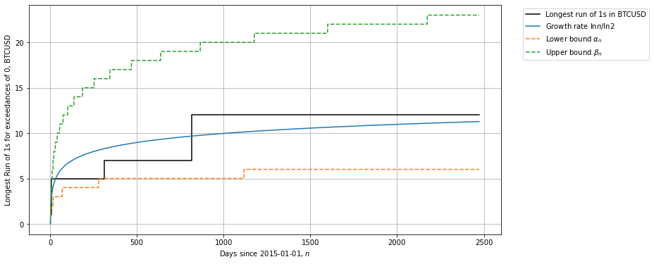
We can see that so far the Bitcoin’s longest streak of 1s (prices closing higher and higher day by day) reached a length of 12 818 days since 2015-01-01 according to Coinbase data. The length is confined between upper and bottom bounds and in agreement with a theoretical growth rate of Erdos and Renyi (1970).

In Sect. 2 the estimated probability of $P(Z_n >= 12)$ in 818 trials was equal 20.97%. Now, you can see why we did it.