There is no question about how profitable the trading of any cryptocurrency can be. If you create an algorithmic strategy and stick to it, you can capture a +10% PnL wave sometimes even twice a day for a selected asset. Unfortunately, the opposite is true, too! The crypto-risks seem to follow the same patterns. But, let’s be optimistic from the beginning.
In this mini-series of articles, we will learn how using Python we can connect to crypto-data provider, process its live stream of OHLC prices, supplement it with an individually-crafted quantitative analysis, estimate the risk levels using VaR and ES metrics, and test mid-frequency trading strategies. A huge benefit of cryptocurrencies is the ease of grabbing the data and earning money given the trading environment 24/7. The number of possibilities is endless, however if you are new to the crypto-world, this series will provide you ample examples on how to kick off your adventure with virtual money.
As a main exchange we will be using Binance. It’s one of the most successful crypto-exchanges, with a very rich Python API and lots of interesting data streamed live as you breath in and breath out. From a quant perspective, it is an excellent laboratory where you can test your trading ideas, mutual data relationships, correlations, apply Python libraries, e.g. ta-lib for technical analysis; ThymeBoost for trend/seasonality/exogenous decomposition and forecasting; or VectorBT for a hyperfast time series analysis, backtesting, and crypto-portfolio optimisation. Sounds exciting? Buckle up! Here we go!
1. An Essential Introduction to Binance Exchange’s Python API and Live Data Streams
Binance Exchange’s offers a solid Python API. The starting webpage here is binance-exchange. Before we begin writing our code, we need to make sure we have installed a websocket_client library. If not, you can quickly keep up the pace by its download and installation as:
$ pip install websocket_client
We also will need a few, rather standard Python libraries, to vouchsafe a smooth execution of the code. Let’s start with typing:
import websocket
import json
import numpy as np
import datetime as dt

SOCKET = 'wss://stream.binance.com:9443/ws/btcusdt@kline_1m'

ws = websocket.WebSocketApp(SOCKET)
ws.run_forever()
First we open a socket pointing at the data stream of our choice. How do we define what data stream we want to use? Well, above, we assumed that we were interested in grabbing BTC/USDT prices broadcasted live with 1-minute frequency. The webpage of Web Socket Streams (WSS) for Binance provides a user with all essential information on the available WSS. We can see that the base endpoint is wss://stream.binance.com:9443. Streams can be accessed either in a single raw stream or in a combined stream where the raw streams are accessed at /ws/
2. Capturing Data from the Stream
The stream is dead unless we take some action. We need to specify a few functions which will be called directly by websocket in line #12. Let’s rewrite this function to a more functional form as follows:
ws = websocket.WebSocketApp(SOCKET, on_open=on_open, on_close=on_close, on_message=on_message)
Now, we need tell what to do “on open” of the connection and “on close” of it:
def on_open(ws):
    return 'opened connection'

def on_close(ws):
    return 'closed connection'
The input parameters here are ws (websocket) but the functions can return rather irrelevant information we can see above. Next, we also need to define some variables:
PROJECT_PATH = '/Users/pawel/Projects/vs'
DATA_PATH = '/data/'
DATA_FILENAME = 'btc_usdt_1m_20220321_set01'

ne = 0  # number of events per candle
database = {}  # a local data storage
j = 0  # a local counter
which are rather self-explanatory. Inside Python dictionary of database we are going to save the data from the stream. Of course, it’s not the best practice but for the sake of this task it’s sufficient enough.
Next, let’s have a second look at the output from the stream as given at this webpage, i.e.
{
  "e": "kline",     // Event type
  "E": 123456789,   // Event time
  "s": "BNBBTC",    // Symbol
  "k": {
    "t": 123400000, // Kline start time
    "T": 123460000, // Kline close time
    "s": "BNBBTC",  // Symbol
    "i": "1m",      // Interval
    "f": 100,       // First trade ID
    "L": 200,       // Last trade ID
    "o": "0.0010",  // Open price
    "c": "0.0020",  // Close price
    "h": "0.0025",  // High price
    "l": "0.0015",  // Low price
    "v": "1000",    // Base asset volume
    "n": 100,       // Number of trades
    "x": false,     // Is this kline closed?
    "q": "1.0000",  // Quote asset volume
    "V": "500",     // Taker buy base asset volume
    "Q": "0.500",   // Taker buy quote asset volume
    "B": "123456"   // Ignore
  }
}
The minimum information we will be satisfied to grab from this stream is:
  "E": 123456789, // Event time
  "t": 123400000, // Kline start time
  "T": 123460000, // Kline close time
  "o": "0.0010",  // Open price
  "c": "0.0020",  // Close price
  "h": "0.0025",  // High price
  "l": "0.0015",  // Low price
  "x": false,     // Is this kline closed?
At the first glance, the event time is provided by some internal, continuous time measure. A handy method to convert it to a Gregorian timestamp is:
def convtime(t, corr=True):
    if corr:
        t = t / 1000
    return dt.datetime.fromtimestamp(t).strftime("%Y-%m-%d %H:%M:%S")
which employs standard Python library of datetime. The Kline start time and Kline close time refer to the beginning and end time-point of 1-minute candlestick, respectively. The variable of x seems to be a key information, i.e. whether the candlestick is officially closed or still… in the process of its formation. As we are going to see in Part 2, this element of the stream opens up a new dimension of live data analysis for algo-trading purposes!
Equipped with all fundamental knowledge, we are ready to write the final form of the on_message function. Let’s put our entire code together:
# Hacking 1-Minute Cryptocurrency Candlesticks: (1) Capturing Binance Exchange Live Data Stream
# (c) 2022 by QuantAtRisk.com
#
# File name: data_download.py

import websocket
import json
import numpy as np
import datetime as dt

SOCKET = 'wss://stream.binance.com:9443/ws/btcusdt@kline_1m'
PROJECT_PATH = '/Users/pawel/Projects/vs'
DATA_PATH = '/data/'
DATA_FILENAME = 'btc_usdt_1m_20220321_set01'

ne = 0  # number of events per candle
database = {}  # a local data storage
j = 0  # a local counter

def convtime(t, corr=True):
    if corr:
        t = t / 1000
    return dt.datetime.fromtimestamp(t).strftime("%Y-%m-%d %H:%M:%S")

def on_open(ws):
    return 'opened connection'

def on_close(ws):
    return 'closed connection'

def on_message(ws, message):
    global ne, j, database

    msg = json.loads(message)
    if msg is not None:

        # save a new candle (interim and final)
        database[str(j)] = msg
        json.dump(database, open(PROJECT_PATH + DATA_PATH + DATA_FILENAME + '.json', 'w'))
        j = j + 1

        et, t1, t2, o, h, l, c, x = msg['E'], msg['k']['t'], msg['k']['T'],
                                    float(msg['k']['o']), float(msg['k']['h']),
                                    float(msg['k']['l']), float(msg['k']['c']),
                                    msg['k']['x']
        if x:
            print(ne)
            ne = 0
            print()
            print('%s %s %s %.2f %.2f %.2f %.2f %s %3g' % (convtime(et),
                         convtime(t1), convtime(t2), o, h, l, c, x, ne))
            print()
        else:
            ne = ne + 1
            print('%s %s %s %.2f %.2f %.2f %.2f %s %3g' % (convtime(et),
                         convtime(t1), convtime(t2), o, h, l, c, x, ne))


# create a new websocket
ws = websocket.WebSocketApp(SOCKET, on_open=on_open, on_close=on_close, on_message=on_message)
ws.run_forever()
When executed, the exemplary output may look like:
2022-03-21 21:14:21 2022-03-21 21:14:00 2022-03-21 21:14:59 41195.18 41204.85 41195.17 41196.36 False   1
2022-03-21 21:14:24 2022-03-21 21:14:00 2022-03-21 21:14:59 41195.18 41204.85 41195.17 41196.35 False   2
2022-03-21 21:14:26 2022-03-21 21:14:00 2022-03-21 21:14:59 41195.18 41204.85 41195.17 41196.36 False   3
2022-03-21 21:14:29 2022-03-21 21:14:00 2022-03-21 21:14:59 41195.18 41204.85 41195.17 41196.36 False   4
2022-03-21 21:14:31 2022-03-21 21:14:00 2022-03-21 21:14:59 41195.18 41204.85 41195.17 41196.35 False   5
2022-03-21 21:14:33 2022-03-21 21:14:00 2022-03-21 21:14:59 41195.18 41204.85 41195.17 41196.35 False   6
2022-03-21 21:14:35 2022-03-21 21:14:00 2022-03-21 21:14:59 41195.18 41204.85 41195.17 41196.36 False   7
...
You can verify quickly that the number of events (streamed by Binance socket) per individual candlestick is not constant and varies by a small amount. It’s nothing wrong, no one told us it should be constant.
Please note that as long as the code is running (remember: forever!) new data streamed are concurrently saved in btc_usdt_1m_20220321_set01.json file.
3. Live Preview of Captured Data
If you allow to run data_download.py hosting the above code in one Terminal window, there is way to execute the “data preview” code as a separate instance. For R&D purposes, I would recommend scripting and running it in Jupyter Notebook but it’s just one option. First, we need to load the current content of the btc_usdt_1m_20220321_set01.json file and next convert it, best, to pandas’ DataFrame for a better data handling:
# Hacking 1-Minute Cryptocurrency Candlesticks: (1) Capturing Binance Exchange Live Data Stream
# (c) 2022 by QuantAtRisk.com
#
# File name: preview_candles.py
import numpy as np
import pandas as pd
import json
import datetime
from pprint import pprint as pp
import plotly.graph_objects as go # for candlestick charts
import matplotlib.dates as mdates
import matplotlib.pyplot as plt
PROJECT_PATH = '/Users/pawel/Projects/vs'
DATA_PATH = '/data/'
DATA_FILENAME = 'btc_usdt_1m_20220321_set01'
# color codes for plotly
whiteP, blackP, redP, greyP = '#FFFFFF', '#000000', '#B54D47', 'rgb(150,150,150)'
def convtime(t, corr=True):
if corr:
t = t / 1000
return datetime.datetime.fromtimestamp(t).strftime("%Y-%m-%d %H:%M:%S")
# read database
data = json.load( open(PROJECT_PATH + DATA_PATH + DATA_FILENAME + '.json') )
keys = list(data.keys())
df = pd.DataFrame(columns=['Timestamp', 'Event_Time', 'Candle_Start', 'Candle_End',
'Freq', 'Open', 'High', 'Low', 'Close', 'Final'])
for k in data.keys():
ts = data[k]['E'] # timestamp
o, h, l, c = float(data[k]['k']['o']), float(data[k]['k']['h']), f
loat(data[k]['k']['l']), float(data[k]['k']['c'])
freq, final = data[k]['k']['i'], data[k]['k']['x']
event_time = convtime(ts)
c_start, c_end = convtime(data[k]['k']['t']), convtime(data[k]['k']['T'])
df.loc[len(df)] = [ts, event_time, c_start, c_end, freq, o, h, l, c, final]
df.set_index(['Timestamp'], drop=True, inplace=True)
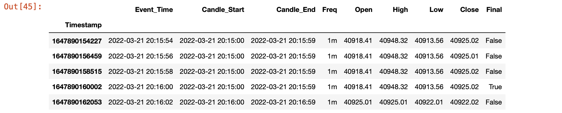
# display first five-rows of 'df'
df.head()
At this stage, we can see the effect of data conversion as:
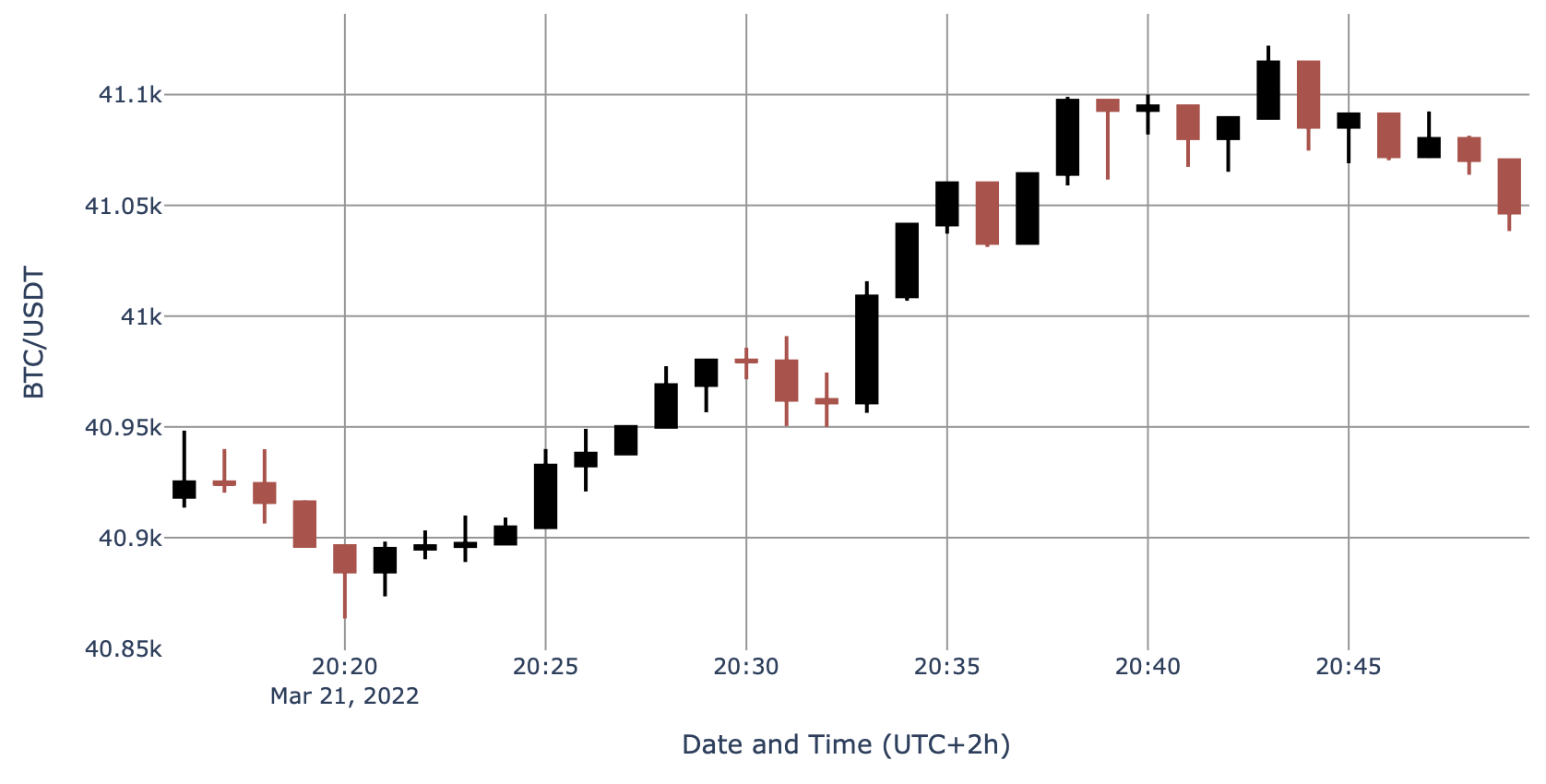
or visualized using the remaining part of the code:
# plot only final candlestick values of OHLC
dff = df[df['Final'] == True]

# chart
fig = go.Figure(data=go.Candlestick(x     = dff.iloc[:,0],
                                    open  = dff.iloc[:,4],
                                    high  = dff.iloc[:,5],
                                    low   = dff.iloc[:,6],
                                    close = dff.iloc[:,7],)
               )
fig.update(layout_xaxis_rangeslider_visible=False)
fig.update_layout(plot_bgcolor=whiteP, width=900)
fig.update_xaxes(showgrid=True, gridwidth=1, gridcolor=greyP)
fig.update_yaxes(showgrid=True, gridwidth=1, gridcolor=greyP)
fig.update_yaxes(title_text='BTC/USDT')
fig.update_xaxes(title_text='Date and Time (UTC+2h)')

# update line and fill colors
cs = fig.data[0]
cs.increasing.fillcolor, cs.increasing.line.color = blackP, blackP
cs.decreasing.fillcolor, cs.decreasing.line.color = redP, redP

fig.show()
delivering the finalized (closed) 1-minute candlesticks of BTC/USDT pair as traded at Binance Crypto-Exchange:
NEXT TIME
In Part 2 in this series, we will dive into the inner structure of each candlestick and develop some tools for the analysis of OHLC prices, time-depended statistics, and properties. We will examine how this new knowledge can trigger the development of mid-frequency algo-trading model.
1 comment