Everybody would agree on one thing: the nervousness among traders may lead to massive sells of stocks, the avalanche of prices, and huge losses. We have witnessed this sort of behaviour many times. An anxiety is the feeling of uncertainty, a human inborn instinct that triggers a self-defending mechanism against high risks. The apex of anxiety is fear and panic. When the fear spreads among the markets, all goes south. It is a dream goal for all traders to capture the nervousness and fear just by looking at or studying the market behaviour, trading patterns, ask-bid spread, or flow of orders. The major problem is that we know very well how much a human behaviour is an important factor in the game but it is not observed directly. It has been puzzling me for a few years since I accomplished reading Your Money and Your Brain: How the New Science of Neuroeconomics Can Help Make You Rich by Jason Zweig sitting at the beach of one of the Gili Islands, Indonesia, in December of 2009. A perfect spot far away from the trading charts.
So, is there a way to disentangle the emotional part involved in trading from all other factors (e.g. the application of technical analysis, bad news consequences, IPOs, etc.) which are somehow easier to deduce? In this post I will try to make a quantitative attempt towards solving this problem. Although the solution will not have the final and closed form, my goal is to deliver an inspiration for quants and traders interested in the subject by putting a simple idea into practice: the application of Principal Component Analysis.
1. Principal Component Analysis (PCA)
Called by many as one of the most valuable results from applied linear algebra, the Principal Component Analysis, delivers a simple, non-parametric method of extracting relevant information from often confusing data sets. The real-world data usually hold some relationships among their variables and, as a good approximation, in the first instance we may suspect them to be of the linear (or close to linear) form. And the linearity is one of stringent but powerful assumptions standing behind PCA.
Imagine we observe the daily change of prices of $m$ stocks (being a part of your portfolio or a specific market index) over last $n$ days. We collect the data in $\boldsymbol{X}$, the matrix $m\times n$. Each of $n$-long vectors lie in an $m$-dimensional vector space spanned by an orthonormal basis, therefore they are a linear combination of this set of unit length basic vectors: $ \boldsymbol{BX} = \boldsymbol{X}$ where a basis $\boldsymbol{B}$ is the identity matrix $\boldsymbol{I}$. Within PCA approach we ask a simple question: is there another basis which is a linear combination of the original basis that represents our data set? In other words, we look for a transformation matrix $\boldsymbol{P}$ acting on $\boldsymbol{X}$ in order to deliver its re-representation:
$$
\boldsymbol{PX} = \boldsymbol{Y} \ .
$$ The rows of $\boldsymbol{P}$ become a set of new basis vectors for expressing the columns of $\boldsymbol{X}$. This change of basis makes the row vectors of $\boldsymbol{P}$ in this transformation the principal components of $\boldsymbol{X}$. But how to find a good $\boldsymbol{P}$?
Consider for a moment what we can do with a set of $m$ observables spanned over $n$ days? It is not a mystery that many stocks over different periods of time co-vary, i.e. their price movements are closely correlated and follow the same direction. The statistical method to measure the mutual relationship among $m$ vectors (correlation) is achieved by the calculation of a covariance matrix. For our data set of $\boldsymbol{X}$:
$$
\boldsymbol{X}_{m\times n} =
\left[
\begin{array}{cccc}
\boldsymbol{x_1} \\
\boldsymbol{x_2} \\
… \\
\boldsymbol{x_m}
\end{array}
\right]
=
\left[
\begin{array}{cccc}
x_{1,1} & x_{1,2} & … & x_{1,n} \\
x_{2,1} & x_{2,2} & … & x_{2,n} \\
… & … & … & … \\
x_{m,1} & x_{m,2} & … & x_{m,n}
\end{array}
\right]
$$
the covariance matrix takes the following form:
$$
cov(\boldsymbol{X}) \equiv \frac{1}{n-1} \boldsymbol{X}\boldsymbol{X}^{T}
$$ where we multiply $\boldsymbol{X}$ by its transposed version and $(n-1)^{-1}$ helps to secure the variance to be unbiased. The diagonal elements of $cov(\boldsymbol{X})$ are the variances corresponding to each row of $\boldsymbol{X}$ whereas the off-diagonal terms of $cov(\boldsymbol{X})$ represent the covariances between different rows (prices of the stocks). Please note that above multiplication assures us that $cov(\boldsymbol{X})$ is a square symmetric matrix $m\times m$.
All right, but what does it have in common with our PCA method? PCA looks for a way to optimise the matrix of $cov(\boldsymbol{X})$ by a reduction of redundancy. Sounds a bit enigmatic? I bet! Well, all we need to understand is that PCA wants to ‘force’ all off-diagonal elements of the covariance matrix to be zero (in the best possible way). The guys in the Department of Statistics will tell you the same as: removing redundancy diagonalises $cov(\boldsymbol{X})$. But how, how?!
Let’s come back to our previous notation of $\boldsymbol{PX}=\boldsymbol{Y}$. $\boldsymbol{P}$ transforms $\boldsymbol{X}$ into $\boldsymbol{Y}$. We also marked that:
$$
\boldsymbol{P} = [\boldsymbol{p_1},\boldsymbol{p_2},…,\boldsymbol{p_m}]
$$ was a new basis we were looking for. PCA assumes that all basis vectors $\boldsymbol{p_k}$ are orthonormal, i.e. $\boldsymbol{p_i}\boldsymbol{p_j}=\delta_{ij}$, and that the directions with the largest variances are the most principal. So, PCA first selects a normalised direction in $m$-dimensional space along which the variance in $\boldsymbol{X}$ is maximised. That is first principal component $\boldsymbol{p_1}$. In the next step, PCA looks for another direction along which the variance is maximised. However, because of orthonormality condition, it looks only in all directions perpendicular to all previously found directions. In consequence, we obtain an orthonormal matrix of $\boldsymbol{P}$. Good stuff, but still sounds complicated?
The goal of PCA is to find such $\boldsymbol{P}$ where $\boldsymbol{Y}=\boldsymbol{PX}$ such that $cov(\boldsymbol{Y})=(n-1)^{-1}\boldsymbol{XX}^T$ is diagonalised.
We can evolve the notation of the covariance matrix as follows:
$$
(n-1)cov(\boldsymbol{Y}) = \boldsymbol{YY}^T = \boldsymbol{(PX)(PX)}^T = \boldsymbol{PXX}^T\boldsymbol{P}^T = \boldsymbol{P}(\boldsymbol{XX}^T)\boldsymbol{P}^T = \boldsymbol{PAP}^T
$$ where we made a quick substitution of $\boldsymbol{A}=\boldsymbol{XX}^T$. It is easy to prove that $\boldsymbol{A}$ is symmetric. It takes a longer while to find a proof for the following two theorems: (1) a matrix is symmetric if and only if it is orthogonally diagonalisable; (2) a symmetric matrix is diagonalised by a matrix of its orthonormal eigenvectors. Just check your favourite algebra textbook. The second theorem provides us with a right to denote:
$$
\boldsymbol{A} = \boldsymbol{EDE}^T
$$ where $\boldsymbol{D}$ us a diagonal matrix and $\boldsymbol{E}$ is a matrix of eigenvectors of $\boldsymbol{A}$. That brings us at the end of the rainbow.
We select matrix $\boldsymbol{P}$ to be a such where each row $\boldsymbol{p_1}$ is an eigenvector of $\boldsymbol{XX}^T$, therefore
$$
\boldsymbol{P} = \boldsymbol{E}^T .
$$
Given that, we see that $\boldsymbol{E}=\boldsymbol{P}^T$, thus we find $\boldsymbol{A}=\boldsymbol{EDE}^T = \boldsymbol{P}^T\boldsymbol{DP}$ what leads us to a magnificent relationship between $\boldsymbol{P}$ and the covariance matrix:
$$
(n-1)cov(\boldsymbol{Y}) = \boldsymbol{PAP}^T = \boldsymbol{P}(\boldsymbol{P}^T\boldsymbol{DP})\boldsymbol{P}^T
= (\boldsymbol{PP}^T)\boldsymbol{D}(\boldsymbol{PP}^T) =
(\boldsymbol{PP}^{-1})\boldsymbol{D}(\boldsymbol{PP}^{-1})
$$ or
$$
cov(\boldsymbol{Y}) = \frac{1}{n-1}\boldsymbol{D},
$$ i.e. the choice of $\boldsymbol{P}$ diagonalises $cov(\boldsymbol{Y})$ where silently we also used the matrix algebra theorem saying that the inverse of an orthogonal matrix is its transpose ($\boldsymbol{P^{-1}}=\boldsymbol{P}^T$). Fascinating, right?! Let’s see now how one can use all that complicated machinery in the quest of looking for human emotions among the endless rivers of market numbers bombarding our sensors every day.
2. Covariances of NASDAQ, Eigenvalues of Anxiety
We will try to build a simple quantitative model for detection of the nervousness in the trading markets using PCA.
By its simplicity I will understand the following model assumption: no matter what the data conceal, the 1st Principal Component (1-PC) of PCA solution links the complicated relationships among a subset of stocks triggered by a latent factor attributed by us to a common behaviour of traders (human and pre-programmed algos). It is a pretty reasonable assumption, much stronger than, for instance, the influence of Saturn’s gravity on the annual silver price fluctuations. Since PCA does not tell us what its 1-PC means in reality, this is our job to seek for meaningful explanations. Therefore, a human factor fits the frame as a trial value very well.
Let’s consider the NASDAQ-100 index. It is composed of 100 technology stocks. The most current list you can find here: nasdaq100.lst downloadable as a text file. As usual, we will perform all calculations using Matlab environment. Let’s start with data collection and pre-processing:
% Anxiety Detection Model for Stock Traders
%  making use of the Principal Component Analsis (PCA)
%  and utilising publicly available Yahoo! stock data
%
% (c) 2013 QuantAtRisk.com, by Pawel Lachowicz

clear all; close all; clc;


% Reading a list of NASDAQ-100 components
nasdaq100=(dataread('file',['nasdaq100.lst'], '%s', 'delimiter', '\n'))';

% Time period we are interested in
d1=datenum('Jan 2 1998');
d2=datenum('Oct 11 2013');

% Check and download the stock data for a requested time period
stocks={};
for i=1:length(nasdaq100)
    try
        % Fetch the Yahoo! adjusted daily close prices between selected
        % days [d1;d2]
        tmp = fetch(yahoo,nasdaq100{i},'Adj Close',d1,d2,'d');
        stocks{i}=tmp;
        disp(i);
    catch err
        % no full history available for requested time period
    end
end
where, first, we try to check whether for a given list of NASDAQ-100’s components the full data history (adjusted close prices) are available via Yahoo! server (please refer to my previous post of Yahoo! Stock Data in Matlab and a Model for Dividend Backtesting for more information on the connectivity).
The cell array stocks becomes populated with two-dimensional matrixes: the time-series corresponding to stock prices (time,price). Since the Yahoo! database does not contain a full history for all stocks of our interest, we may expect their different time spans. For the purpose of demonstration of the PCA method, we apply additional screening of downloaded data, i.e. we require the data to be spanned between as defined by $d1$ and $d2$ variables and, additionally, having the same (maximal available) number of data points (observations, trials). We achieve that by:
% Additional screening
d=[];
j=1;
data={};
for i=1:length(nasdaq100)
    d=[d; i min(stocks{i}(:,1)) max(stocks{i}(:,1)) size(stocks{i},1)];
end
for i=1:length(nasdaq100)
    if(d(i,2)==d1) && (d(i,3)==d2) && (d(i,4)==max(d(:,4)))
        data{j}=sortrows(stocks{i},1);
        fprintf('%3i %1s\n',i,nasdaq100{i})
        j=j+1;
    end
end
m=length(data);
The temporary matrix of $d$ holds the index of stock as read in from nasdaq100.lst file, first and last day number of data available, and total number of data points in the time-series, respectively:
>> d
d =
      1      729757      735518        3970
      2      729757      735518        3964
      3      729757      735518        3964
      4      729757      735518        3969
     ..          ..          ..          ..
     99      729757      735518        3970
    100      729757      735518        3970
Our screening method saves $m=21$ selected stock data into data cell array corresponding to the following companies from our list:
  1 AAPL
  7 ALTR
  9 AMAT
 10 AMGN
 20 CERN
 21 CHKP
 25 COST
 26 CSCO
 30 DELL
 39 FAST
 51 INTC
 64 MSFT
 65 MU
 67 MYL
 74 PCAR
 82 SIAL
 84 SNDK
 88 SYMC
 96 WFM
 99 XRAY
100 YHOO
Okay, some people say that seeing is believing. All right. Let’s see how it works. Recall the fact that we demanded our stock data to be spanned between ‘Jan 2 1998’ and ‘Oct 11 2013’. We found 21 stocks meeting those criteria. Now, let’s assume we pick up a random date, say, Jul 2 2007 and we extract for all 21 stocks their price history over last 90 calendar days. We save their prices (skipping the time columns) into $Z$ matrix as follows:
t=datenum('Jul 2 2007');
Z=[];
for i=1:m
    [r,c,v]=find((data{i}(:,1)<=t) & (data{i}(:,1)>t-90));
    Z=[Z data{i}(r,2)]
end
and we plot them all together:
plot(Z)
xlim([1 length(Z)]);
ylabel('Stock price (US$)');
xlabel('T-90d');
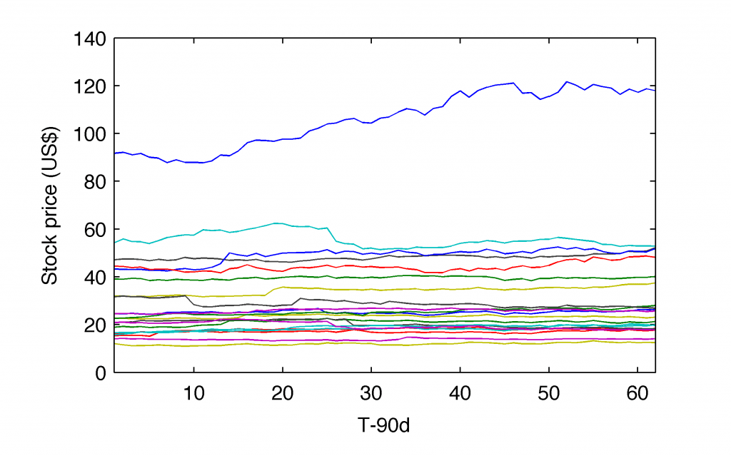
It’s easy to deduct that the top one line corresponds to Apple, Inc. (AAPL) adjusted close prices.
The unspoken earlier data processing methodology is that we need to transform our time-series into the comparable form. We can do it by subtracting the average value and dividing each of them by their standard deviations. Why? For a simple reason of an equivalent way of their mutual comparison. We call that step a normalisation or standardisation of the time-series under investigation:
[N,M]=size(Z);
X=(Z-repmat(mean(Z),[N 1]))./repmat(std(Z),[N 1]);
This represents the matrix $\boldsymbol{X}$ that I discussed in a theoretical part of this post. Note, that the dimensions are reversed in Matlab. Therefore, the normalised time-series,
% Display normalized stock prices
plot(X)
xlim([1 length(Z)]);
ylabel('(Stock price-Mean)/StdDev');
xlabel('T-90d');
look like:
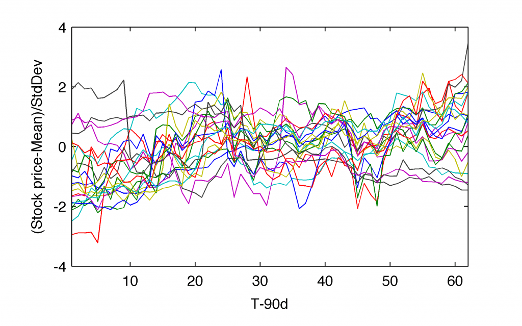
For a given matrix of $\boldsymbol{X}$, its covariance matrix,
% Calculate the covariance matrix, cov(X)
CovX=cov(X);
imagesc(CovX);
as for data spanned 90 calendar day back from Jul 2 2007, looks like:
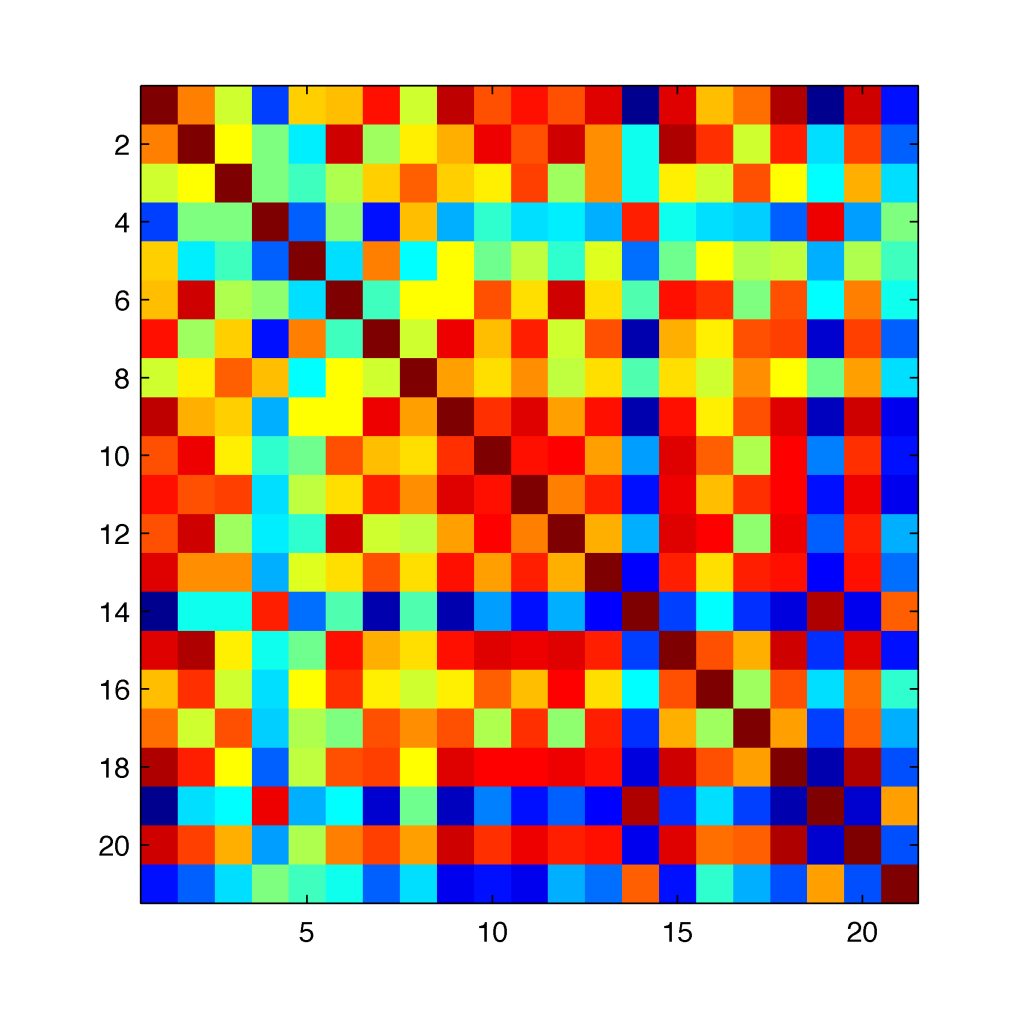
where the colour coding goes from the maximal values (most reddish) down to the minimal values (most blueish). The diagonal of the covariance matrix simply tells us that for normalised time-series, their covariances are equal to the standard deviations (variances) of 1 as expected.
Going one step forward, based on the given covariance matrix, we look for the matrix of $\boldsymbol{P}$ whose columns are the corresponding eigenvectors:
% Find P
[P,~]=eigs(CovX,5);
imagesc(P);
set(gca,'xticklabel',{1,2,3,4,5},'xtick',[1 2 3 4 5]);
xlabel('Principal Component')
ylabel('Stock');
set(gca,'yticklabel',{'AAPL', 'ALTR', 'AMAT', 'AMGN', 'CERN', ...
 'CHKP', 'COST', 'CSCO', 'DELL', 'FAST', 'INTC', 'MSFT', 'MU', ...
 'MYL', 'PCAR', 'SIAL', 'SNDK', 'SYMC', 'WFM', 'XRAY', 'YHOO'}, ...
 'ytick',[1 2 3 4 5 6 7 8 9 10 11 12 13 14 15 16 17 18 19 20 21]);
which results in $\boldsymbol{P}$ displayed as:
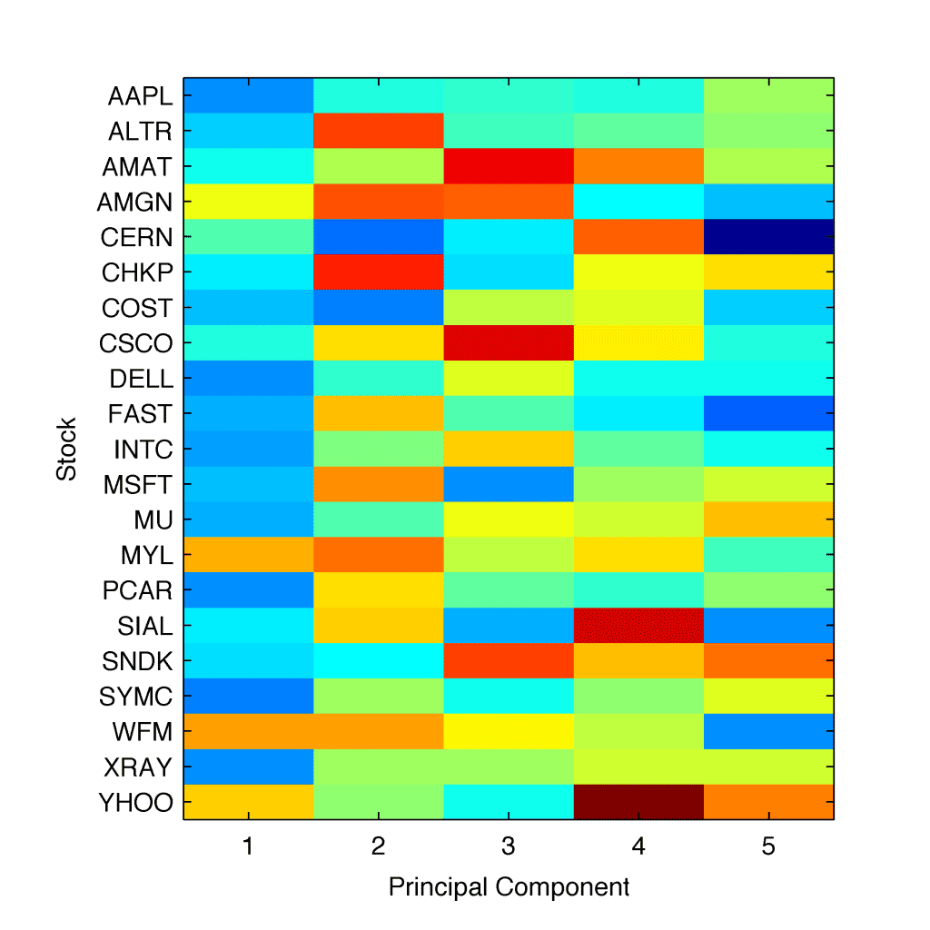
where we computed PCA for five principal components in order to illustrate the process. Since the colour coding is the same as in the previous figure, a visual inspection of of the 1-PC indicates on negative numbers for at least 16 out of 21 eigenvalues. That simply means that over last 90 days the global dynamics for those stocks were directed south, in favour of traders holding short-position in those stocks.
It is important to note in this very moment that 1-PC does not represent the ‘price momentum’ itself. It would be too easy. It represents the latent variable responsible for a common behaviour in the stock dynamics whatever it is. Based on our model assumption (see above) we suspect it may indicate a human factor latent in the trading.
3. Game of Nerves
The last figure communicates an additional message. There is a remarkable coherence of eigenvalues for 1-PC and pretty random patterns for the remaining four principal components. One may check that in the case of our data sample, this feature is maintained over many years. That allows us to limit our interest to 1-PC only.
It’s getting exciting, isn’t it? Let’s come back to our main code. Having now a pretty good grasp of the algebra of PCA at work, we may limit our investigation of 1-PC to any time period of our interest, below spanned between as defined by $t1$ and $t2$ variables:
% Select time period of your interest
t1=datenum('July 1 2006');
t2=datenum('July 1 2010');

results=[];
for t=t1:t2
    tmp=[];
    A=[]; V=[];
    for i=1:m
        [r,c,v]=find((data{i}(:,1)<=t) & (data{i}(:,1)>t-60));
        A=[A data{i}(r,2)];
    end
    [N,M]=size(A);
    X=(A-repmat(mean(A),[N 1]))./repmat(std(A),[N 1]);
    CovX=cov(X);
    [V,D]=eigs(CovX,1);
    % Find all negative eigenvalues of the 1st Principal Component
    [r,c,v]=find(V(:,1)<0);
    % Extract them into a new vector
    neg1PC=V(r,1);
    % Calculate a percentage of negative eigenvalues relative
    % to all values available
    ratio=length(neg1PC)/m;
    % Build a new time-series of 'ratio' change over required
    % time period (spanned between t1 and t2)
    results=[results; t ratio];
end
We build our anxiety detection model based on the change of number of eigenvalues of the 1st Principal Component (relative to the total their numbers; here equal 21). As a result, we generate a new time-series tracing over $[t1;t2]$ time period this variable. We plot the results all in one plot contrasted with the NASDAQ-100 Index in the following way:
% Fetch NASDAQ-100 Index from Yahoo! data-server
nasdaq = fetch(yahoo,'^ndx','Adj Close',t1,t2,'d');
% Plot it
subplot(2,1,1)
plot(nasdaq(:,1),nasdaq(:,2),'color',[0.6 0.6 0.6]);
ylabel('NASDAQ-100 Index');
% Add a plot corresponding to a new time-series we've generated
subplot(2,1,2)
plot(results(:,1),results(:,2),'color',[0.6 0.6 0.6])
% add overplot 30d moving average based on the same data
hold on; plot(results(:,1),moving(results(:,2),30),'b')
leading us to:
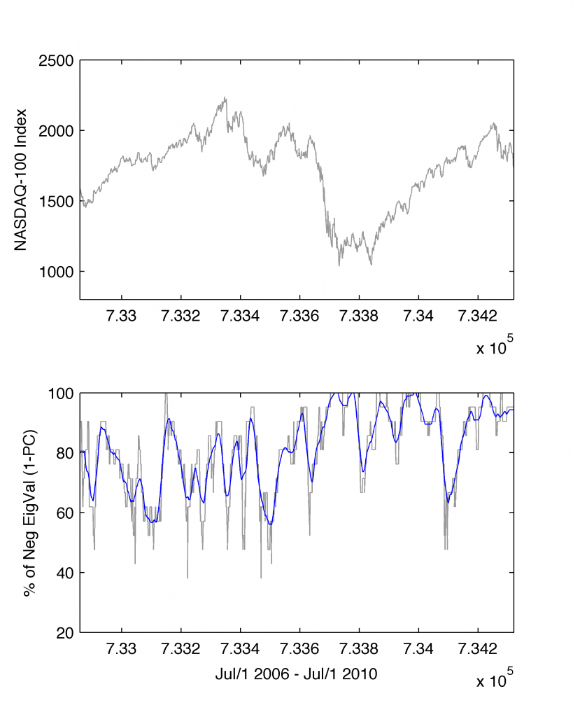
I use 30-day moving average (a solid blue line) in order to smooth the results (moving.m). Please note, that line in #56 I also replaced the earlier value of 90 days with 60 days. Somehow, it is more reasonable to examine with the PCA the market dynamics over past two months than for longer periods (but it’s a matter of taste and needs).
Eventually, we construct the core model’s element, namely, we detect nervousness among traders when the percentage of negative eigenvalues of the 1st Principal Component increases over (at least) five consecutive days:
% Model Core
x1=results(:,1);
y1=moving(results(:,2),30);
tmp=[];
% Find moments of time where the percetage of negative 1-PC
% eigenvalues increases over time (minimal requirement of
% five consecutive days
for i=5:length(x1)
    if(y1(i)>y1(i-1))&&(y1(i-1)>y1(i-2))&&(y1(i-2)>y1(i-3))&& ...
      (y1(i-3)>y1(i-4))&&(y1(i-4)>y1(i-5))
        tmp=[tmp; x1(i)];
    end
end
% When found
z=[];
for i=1:length(tmp)
    for j=1:length(nasdaq)
        if(tmp(i)==nasdaq(j,1))
            z=[z; nasdaq(j,1) nasdaq(j,2)];
        end
    end
end
subplot(2,1,1);
hold on; plot(z(:,1),z(:,2),'r.','markersize',7);
The results of the model we over-plot with red markers on top of the NASDAQ-100 Index:
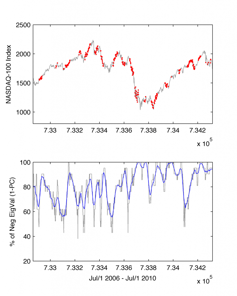
Our simple model takes us into a completely new territory of unexplored space of latent variables. Firstly, it does not predict the future. It still (unfortunately) remains unknown. However, what it delivers is a fresh look at the past dynamics in the market. Secondly, it is easily to read out from the plot that results cluster into three subgroups.
The first subgroup corresponds to actions in the stock trading having further negative consequences (see the events of 2007-2009 and the avalanche of prices). Here the dynamics over any 60 calendar days had been continued. The second subgroup are those periods of time when anxiety led to negative dynamics among stock traders but due to other factors (e.g. financial, global, political, etc.) the stocks surged dragging the Index up. The third subgroup (less frequent) corresponds to instances of relative flat changes of Index revealing a typical pattern of psychological hesitation about the trading direction.
No matter how we might interpret the results, the human factor in trading is evident. Hopefully, the PCA approach captures it. If not, all we are left with is our best friend: a trader’s intuition.
Acknowledgments
An article dedicated to Dr. Dariusz Grech of Physics and Astronomy Department of University of Wroclaw, Poland, for his superbly important! and mind-blowing lectures on linear algebra in the 1998/99 academic year.