In probability and statistics, distributions are often classified as either “thin-tailed” or “fat-tailed,” a distinction that reflects the likelihood of extreme deviations from the mean. The lognormal distribution, however, defies this binary classification. It possesses characteristics that make it neither fully thin-tailed, as in the case of the Gaussian, nor entirely fat-tailed, like the Pareto. This intermediate nature positions the lognormal uniquely in statistical modeling, especially in financial risk analysis and natural sciences.
This article will delve into the lognormal distribution’s characteristics, analyze its tail behavior, and illustrate why it resists categorization as either thin- or fat-tailed. We’ll also include some Python examples to visualize these behaviors and provide a solid understanding of why the lognormal distribution can be challenging to work with in extreme-event modeling.
1. Introduction to the Lognormal Distribution
A variable $Y$ is said to follow a lognormal distribution if it can be expressed as the exponential of a normally distributed variable. Formally, if
$$
X \sim N(\mu, \sigma^2)
$$ then the transformation $ Y = e^X$ results in $Y$ following a lognormal distribution with parameters $\mu$ and $\sigma$, denoted as $Y \sim \mbox{Lognormal} (\mu, \sigma^2)$.
The probability density function (PDF) of the lognormal distribution is given by:
$$
f_Y(y) = \frac{1}{y \sigma \sqrt{2\pi}} \exp \left( -\frac{(\ln y – \mu)^2}{2\sigma^2} \right), \quad y > 0.
$$ Unlike the Gaussian, which is symmetric and extends infinitely in both directions, the lognormal is strictly positive ($y > 0$) and exhibits a right-skewed, asymmetric shape. This reflects its relevance in modeling quantities that cannot be negative, such as stock prices, biological measurements, or income distributions.
2. Thin vs. Fat Tails: Conceptual Differences
Before examining where the lognormal fits, let’s distinguish between thin- and fat-tailed distributions:
Thin-tailed distributions like the Gaussian exhibit rapid decay in their tails, meaning extreme values (those far from the mean) are increasingly unlikely. In mathematical terms, for a thin-tailed random variable $Z$ with PDF $f_Z(z)$, we have:
$$
\lim_{z \to \infty} \frac{f_Z(z + x)}{f_Z(z)} = 0 \quad \text{for any fixed } x > 0.
$$ This implies that extreme deviations are exceedingly rare and, consequently, have minimal impact on overall statistical properties. On the other hand, fat-tailed distributions, such as the Pareto, decay more slowly in their tails, implying a higher likelihood of extreme values. For a fat-tailed random variable $W$ with PDF $f_W(w)$, the tails behave according to a power law:
$$
P(W > w) \sim w^{-\alpha} \quad \text{for some } \alpha > 0.
$$ Here, the rate of decay is polynomial, which allows for extreme values to have a significant influence on the distribution’s mean, variance, and other higher-order moments (often leading to their non-existence).
The lognormal, as we will explore, does not strictly adhere to either of these behaviors, exhibiting a unique subexponential decay in its tail probabilities.
3. Lognormal’s “In-Between” Behavior: Neither Thin Nor Fat
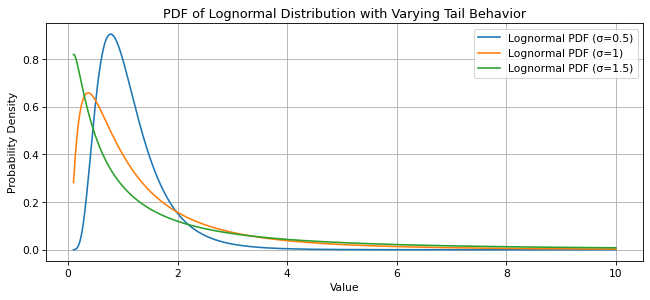
While not exactly fat-tailed, the lognormal distribution also cannot be classified as thin-tailed due to its slow decay. This becomes clearer when examining the right tail of the lognormal. For large values of $y$, the PDF of the lognormal approximates as:
$$
f_Y(y) \approx \frac{1}{y^{1 + \sigma^2 / (2\mu)}}.
$$ This decay is faster than a power law (which would make it fat-tailed) but slower than exponential, meaning it has properties of both thin- and fat-tailed distributions depending on the variance $\sigma^2$. As $\sigma$ grows, the lognormal’s tail becomes heavier and more closely resembles a fat tail:
import numpy as np
import matplotlib.pyplot as plt
from scipy.stats import lognorm

# Parameters for lognormal distribution
mu = 0
sigma_values = [0.5, 1, 1.5]  # Different variances for lognormal

# Range of values for plotting
x = np.linspace(0.1, 10, 1000)

# Plotting the PDF of lognormal with varying sigma
plt.figure(figsize=(10, 4), dpi=77)

for sigma in sigma_values:
    scale = np.exp(mu)
    pdf_values = lognorm.pdf(x, sigma, scale=scale)
    plt.plot(x, pdf_values, label=f'Lognormal PDF (σ={sigma})')

plt.xlabel('Value')
plt.ylabel('Probability Density')
plt.title('PDF of Lognormal Distribution with Varying Tail Behavior')
plt.legend()
plt.grid(True)

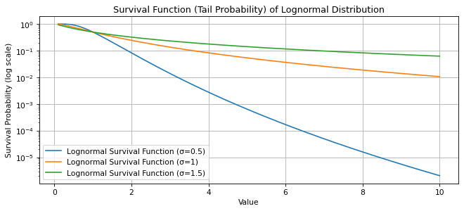
To quantify this tail behavior, we can use Karamata’s characterization of regularly varying functions. For a distribution with a survival function $\bar{F}(y) = P(Y > y)$, the lognormal’s survival function decays such that:
$$
\bar{F}(y) = P(Y > y) \sim \frac{1}{y \log(y)}, \quad y \rightarrow \infty.
$$ This rate of decay situates the lognormal as subexponential, meaning its extreme values are not as frequent as in fat-tailed distributions but occur more frequently than in thin-tailed ones. This approximation describes the probability that a lognormal variable exceeds a high threshold $y$. Unlike the Gaussian survival function, which decays exponentially, the lognormal’s survival function decays at a rate between exponential and polynomial, meaning that large deviations are not as rare as in thin-tailed distributions but not as frequent as in fat-tailed distributions like the Pareto.
# Parameters for lognormal distribution
mu = 0
sigma_values = [0.5, 1, 1.5]  # Different variances for lognormal

# Range of values for plotting
x = np.linspace(0.1, 10, 1000)

# Plotting the Survival Function of lognormal with varying sigma
plt.figure(figsize=(10, 4), dpi=77)

for sigma in sigma_values:
    scale = np.exp(mu)
    survival_values = 1 - lognorm.cdf(x, sigma, scale=scale)
    plt.plot(x, survival_values, label=f'Lognormal Survival Function (σ={sigma})')

plt.yscale('log')  # Logarithmic scale for better visualization of tail decay
plt.xlabel('Value')
plt.ylabel('Survival Probability (log scale)')
plt.title('Survival Function (Tail Probability) of Lognormal Distribution')
plt.legend()
plt.grid(True)
4. Moments and the Challenges of Lognormal
The moment behavior of the lognormal further distinguishes it from thin-tailed distributions.
- Finite Expected Value: For any lognormal random variable, $Y$, the mean is given by $\mathbb{E}[Y] = e^{\mu + \sigma^2 / 2}.$ This is always finite, regardless of the variance $\sigma^2$, making it unlike some fat-tailed distributions where even the mean can diverge.
- Finite Variance: The variance is also finite, calculated as $\text{Var}(Y) = (e^{\sigma^2} – 1) e^{2\mu + \sigma^2}$. However, as $\sigma \rightarrow \infty$ the variance increases exponentially, indicating a sensitivity to extreme deviations.
-
Higher Moments: Higher-order moments, such as skewness and kurtosis, grow rapidly with $\sigma$, reflecting an increasing tail thickness. For instance, the $k$-th moment is
$$
\mathbb{E}[Y^k] = e^{k\mu + k^2 \sigma^2 / 2}.
$$ As $k$ increases, so does the moment, at an exponential rate dependent on $\sigma$, underscoring the lognormal’s tendency toward higher extremes.
The presence of finite mean and variance aligns it with thin tails, yet the explosive growth in higher moments suggests some influence from fat tails, especially as $\sigma$ grows large.
5. Lognormal and Subexponentiality
A notable property of the lognormal is its subexponential behavior, often discussed in the context of heavy tails. The subexponential class, to which the lognormal belongs, satisfies:
$$
\lim_{y \to \infty} \frac{\bar{F}^{*2}(y)}{\bar{F}(y)} = 2.
$$ where $ \bar{F}^{*2}(y) $ epresents the survival function of the sum of two independent lognormal variables. In simple terms, the probability of a large deviation in the sum of two lognormal variables is close to twice the probability of a large deviation in either of the two individual variables.
For a fully fat-tailed distribution, the largest extreme value typically dominates the sum, while in thin-tailed distributions, the sum behaves more predictably. The lognormal’s placement in this in-between state implies that while the sum may be dominated by one large deviation, it does not have the same outsized effect seen in fat-tailed distributions.
6. Quick Note on Applications
Since lognormal distributions account for positive skewness (higher chance of large positive returns), they are useful for modeling portfolio returns. However, the unpredictability introduced by its tail structure complicates precise risk estimates, particularly for VaR (Value at Risk) calculations, which might underestimate risks if only thin-tailed models are assumed.
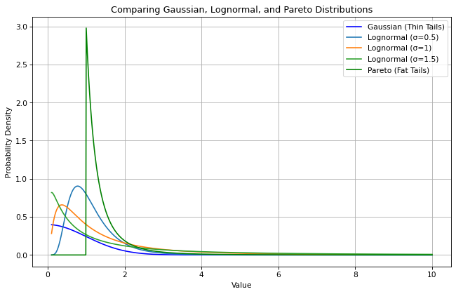
In order to visualize the lognormal distribution alongside Gaussian and Pareto distributions to understand how the lognormal’s tail differs from classic thin- and fat-tailed behaviors one can code it as follows:
# Parameters for distributions
mu = 0
sigma_values = [0.5, 1, 1.5]  # Varying sigma to show tail heaviness for lognormal
alpha = 3  # Tail index for Pareto

x = np.linspace(0.1, 10, 1000)

# Plotting
plt.figure(figsize=(10, 6), dpi=77)

# Gaussian for reference
plt.plot(x, norm.pdf(x, mu, 1), label='Gaussian (Thin Tails)', color='blue')

# Lognormals with increasing σ
for sigma in sigma_values:
    scale = np.exp(mu)
    plt.plot(x, lognorm.pdf(x, sigma, scale=scale), label=f'Lognormal (σ={sigma})')

# Pareto for fat tail reference
plt.plot(x, pareto.pdf(x, alpha), label=f'Pareto (Fat Tails)', color='green')

plt.xlabel('Value')
plt.ylabel('Probability Density')
plt.title('Comparing Gaussian, Lognormal, and Pareto Distributions')
plt.legend()
plt.grid(True)
what gives us

Here, the Gaussian exhibits rapid decay and a predictable center, showing thin tails; the lognormal reveals that the tail grows heavier as $\sigma$ increases, indicating a heavier tail but not as extreme as the Pareto; and as for Pareto, it displays the slowest decay, indicating the highest probability of extreme values.
The lognormal distribution’s “in-between” nature makes it a flexible yet challenging tool in statistical modeling. It straddles the boundary between thin- and fat-tailed distributions, making it difficult to classify yet valuable for modeling real-world phenomena. While useful for predicting typical behaviors, its tail behavior should be handled cautiously, especially in risk-sensitive domains where extreme values have substantial impacts.
