Conditional Value-at-Risk (CVaR), also referred to as the Expected Shortfall (ES) or the Expected Tail Loss (ETL), has an interpretation of the expected loss (in present value terms) given that the loss exceeds the VaR (e.g. Alexander 2008). For many risk analysts, Conditional Value-at-Risk makes more sense: if VaR is a “magical” threshold, the CVaR provides us with more intuitive expectation of how much we will lose if the asset drops in trading (over next $h$ days) below a pre-calculated VaR. The underlying model for VaR is directly linked to the daily return distribution for the asset (or portfolio) by the best fit.
In my previous post, Student t Distributed Linear Value-at-Risk, we have compared the VaRs coming from two fitted distributions: Normal and Student $t$. The key point was related to the left (fat or not) tails: the devil playing with us. If the asset displays a greater number of heavy losses, a standard procedure of fitting the overall daily return distribution with the Normal distribution simply underestimates the left tail (i.e., the model is wrong). We have seen that Student $t$ distribution could be an appealing alternative (i.e., a much better model). Both VaRs differs, so Conditional Value-at-Risk should too.
Today, let’s see how one can derive Conditional Value-at-Risk for Normal and Student $t$ distribution, respectively, and compare them using a real data for the IBM stock traded at New York Stock Exchange (NYSE).
1. VaR and Conditional Value-at-Risk
If $X$ represents the $h$-day returns then $\mbox{VaR}_{h, \alpha} = -x_{h, \alpha}$ where $P(X < x_{h, \alpha}) = \alpha$. Keeping that in mind, the Conditional Value-at-Risk, expressed as a percentage of the portfolio value, is given by:
$$
\mbox{CVaR}_{h, \alpha} (X) = -E(X | X < x_{h, \alpha}) = -\alpha^{-1} \int_{-\infty}^{x_{h, \alpha}} xf(x)\ dx .
$$ Therefore, in order to derive Conditional Value-at-Risk for any continuous probability density function of $f(x)$, we need to integrate $xf(x)$ over $x$ till $100(1-\alpha)$%$h$-day VaR (i.e. $x_{h, \alpha}$ quantile). Now, one can find that:
$$
\mbox{CVaR}_{h, \alpha} (X) = \alpha^{-1} \varphi(\Phi^{-1}(\alpha))\sigma_h – \mu_h
$$ is CVaR in the normal linear VaR model for a random variable $X\sim N(\mu_h, \sigma_h^2)$ over $h$-day horizon where $\varphi(z)$ denotes the standard normal density function and $\Phi^{-1}(\alpha)$ the $\alpha$ quantile of the standard normal distribution.
Since maths can be exciting, more excitement comes from a practical example. Suppose that we wish to find 5-day CVaR for a stock characterised by its annual expected volatility of $\sigma = 41\%$ at $\mu = 0$. Therefore, the 5-day standard deviation we find as $\sigma_h = \sigma_{h=5} = \sigma \sqrt{h/252} = 0.41\sqrt{5/252} = 0.05798$ assuming 252 trading days in a calendar year and $\alpha=0.01$ significance level. Next, deriving in Python,
h = 5
mu_h = 0
sig_h = 0.41 * np.sqrt(h/252)
alpha = 0.01
lev = 100*(1-alpha)

CVaR_n = alpha**-1 * norm.pdf(norm.ppf(alpha))*sig_h - mu_h
VaR_n = norm.ppf(1-alpha)*sig_h - mu_h

print("%g%% %g-day Normal CVaR   = %.2f%%" % (lev, h, CVaR_n *100))
print("%g%% %g-day Normal VaR    = %.2f%%" % (lev, h, VaR_n*100))
we get
99% 5-day Normal CVaR   = 15.45%
99% 5-day Normal VaR    = 13.49%
Again, if the stock in 5 days loses more than $13.49\%$ and we hold it in our portfolio, in fact, we expect the loss greater than VaR which is CVaR of $15.45\%$. All right, but what if the stock daily returns, especially the far left end of their distribution, can be better modelled by fitting Student $t$ pdf rather than Normal pdf function? We need to find the way to express CVaR for Student $t$ distribution.
The standardised Student $t$ distribution is given by its probability density function:
$$
f_\nu(x) = \underbrace{((\nu-2)\pi)^{-1/2} \Gamma\left(\frac{\nu}{2}\right)^{-1} \Gamma\left(\frac{\nu+1}{2}\right)}_\text{A}
(1+ \underbrace{(\nu-2)^{-1}}_\text{a} x^2)^{\overbrace{-(\nu+1)/2}^\text{b}}
$$ where $\Gamma$ denotes the gamma function and $\nu$ the degrees of freedom, and reduces to:
$$
f_\nu(x) = A(1+ax^2)^b \ .
$$ Engaging the integral definition for Conditional Value-at-Risk we derive:
$$
\mbox{CVaR}_{\alpha, \nu} = -\alpha^{-1} \int_{-\infty}^{x_{\alpha, \nu}} xf_\nu(x)\ dx =
-\alpha^{-1} \int_{-\infty}^{x_{\alpha, \nu}} x A(1+ax^2)^b dx \\
= -\frac{A}{\alpha} \int_{-\infty}^{x_{\alpha, \nu}} x (\underbrace{1+ax^2}_\text{y})^b dx
$$ followed by ${\mathrm d}y = 2a{\mathrm d}x$ thus ${\mathrm d}x = {\mathrm d}y/2ax$, so:
$$
= -\frac{A}{\alpha} \int_{-\infty}^{B} \frac{x(1+ax)^b}{2ax} {\mathrm d}y \ .
$$ Given $y = 1+ax^2$ and $a$ above, we denote $B = 1 + (\nu-2)^{-1} x^2_{\alpha, \nu}$. Continuing,
$$
= -\frac{A}{2a\alpha} \int_{-\infty}^{B} y^b {\mathrm d}y =
-\frac{A}{2a\alpha} \frac{B^{b+1}}{b+1} \ .
$$ Since $b+1 = -(\nu+1)/2 + 1 = (1-\nu)/2$ then:
$$
= -\frac{A}{(\nu-2)^{-1}\alpha} \frac{2B^{(1-\nu)/2}}{(1-\nu)}
$$ and noting that:
$$
f_\nu(x) = A ( \underbrace{ 1 + (\nu-2)^{-1} x^2_{\alpha, \nu} }_\text{B} )^b \\
f_\nu(x) = A B^b \\
A = f_\nu(x) B^{-b} = f_\nu(x) B^{(1+\nu)/2}
$$ we derive Conditional Value-at-Risk further:
$$
= -\alpha^{-1} \frac{ f_\nu(x) B^{(1+\nu)/2} }{2(\nu-2)^{-1}} \frac{2B^{(1-\nu)/2}}{(1-\nu)} =
-\alpha^{-1} f_\nu(x) (\nu-2) (1-\nu)^{-1} B
$$
$$
= -\alpha^{-1} (\nu-2) (1-\nu)^{-1} (1 + (\nu-2)^{-1} x^2_{\alpha, \nu}) f_\nu(x_{\alpha, \nu})
$$
$$
= -\alpha^{-1} (1-\nu)^{-1} [\nu-2 + x^2_{\alpha, \nu}] f_\nu(x_{\alpha, \nu})
$$ Eventually, $h$-day CVaR in Student t Linear VaR Model we can write as:
$$
\mbox{CVaR}_{h, \alpha, \nu} (X) = -\alpha^{-1} (1-\nu)^{-1} [\nu-2 + x^2_{\alpha, \nu}] f_\nu(x_{\alpha, \nu}) \sigma_h – \mu_h \ .
$$ Turning that formula into code, we obtain for, e.g., $\nu=6$ degrees-of-freedom:
h = 10
mu_h = 0
sig = 0.41
sig_h = sig * np.sqrt(h/252)
alpha = 0.01  # significance level
lev = 100*(1-alpha)

nu = 6
xanu = t.ppf(alpha, nu)
CVaR_t = -1/alpha * (1-nu)**(-1) * (nu-2+xanu**2) * t.pdf(xanu, nu)*sig_h - mu_h

VaR_t = np.sqrt(h/252 * (nu-2)/nu) * t.ppf(1-alpha, nu)*sig - mu_norm

print("%g%% %g-day Student t CVaR = %.2f%%" % (lev, h, CVaR_t*100))
print("%g%% %g-day Student t VaR  = %.2f%%" % (lev, h, VaR_t*100))
we get:
99% 10-day Student t CVaR = 28.79%
99% 10-day Student t VaR  = 20.94%
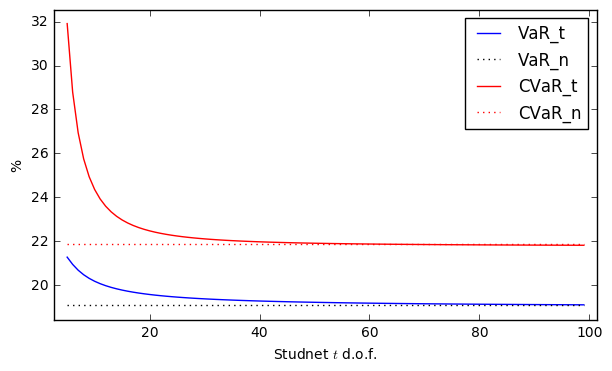
It is easy to show that with an increasing number of degrees-of-freedom for Student $t$ model, the corresponding CVaRs will converge to Conditional Value-at-Risk for the Normal VaR model:
# setup
h = 10
mu_h = 0
sig = 0.41
sig_h = sig * np.sqrt(h/252)
alpha = 0.01  # significance level for Conditional Value-at-Risk
lev = 100*(1-alpha)

d = []
for nu in range(5, 100):
    xanu = t.ppf(alpha, nu)
    CVaR_t = -1/alpha * (1-nu)**(-1) * (nu-2+xanu**2) * \
             t.pdf(xanu, nu)*sig_h - mu_h
    VaR_t = np.sqrt(h/252 * (nu-2)/nu) * t.ppf(1-alpha, nu)*sig \
             - mu_norm
    d.append([nu, VaR_t, CVaR_t])

d = np.array(d).T

fig, ax = plt.subplots(figsize=(7,4))
plt.plot(d[0], d[1]*100, 'b-', label="VaR_t")
plt.plot(np.arange(5, 100), VaR_n*np.ones(95)*100, ":k", label="VaR_n")
plt.plot(d[0], d[2]*100, 'r-', label="CVaR_t")
plt.plot(np.arange(5, 100), CVaR_n*np.ones(95)*100, ":r",label="CVaR_n" )
plt.xlabel("Studnet $t$ d.o.f.")
plt.ylabel("%")
plt.legend(loc=1)
ax.margins(x=0.025, y=0.05) # add extra padding
2. Case Study
Let’s refer to the example for the return-series analysis of the IBM stock in my previous post and run the same code supplemented with Conditional Value-at-Risk calculations:
# Conditional Value-at-Risk in the Normal and Student t Linear VaR Model
# (c) 2016 Pawel Lachowicz, QuantAtRisk.com

import numpy as np
import math
from scipy.stats import skew, kurtosis, kurtosistest
import matplotlib.pyplot as plt
from scipy.stats import norm, t
import pandas_datareader.data as web


# Fetching Yahoo! Finance for IBM stock data
data = web.DataReader("IBM", data_source='yahoo',
                  start='2010-12-01', end='2015-12-01')['Adj Close']
cp = np.array(data.values)  # daily adj-close prices
ret = cp[1:]/cp[:-1] - 1    # compute daily returns

# N(x; mu, sig) best fit (finding: mu, stdev)
mu_norm, sig_norm = norm.fit(ret)
dx = 0.0001  # resolution
x = np.arange(-0.1, 0.1, dx)
pdf = norm.pdf(x, mu_norm, sig_norm)
print("Sample mean  = %.5f" % mu_norm)
print("Sample stdev = %.5f" % sig_norm)
print()

# Student t best fit (finding: nu)
parm = t.fit(ret)
nu, mu_t, sig_t = parm
nu = np.round(nu)
pdf2 = t.pdf(x, nu, mu_t, sig_t)
print("nu = %.2f" % nu)
print()

# Compute VaRs and Conditional Value-at-Risk

h = 1
alpha = 0.01  # significance level
lev = 100*(1-alpha)
xanu = t.ppf(alpha, nu)

CVaR_n = alpha**-1 * norm.pdf(norm.ppf(alpha))*sig_norm - mu_norm
VaR_n = norm.ppf(1-alpha)*sig_norm - mu_norm

VaR_t = np.sqrt((nu-2)/nu) * t.ppf(1-alpha, nu)*sig_norm  - h*mu_norm
CVaR_t = -1/alpha * (1-nu)**(-1) * (nu-2+xanu**2) * \
                t.pdf(xanu, nu)*sig_norm  - h*mu_norm

print("%g%% %g-day Normal VaR     = %.2f%%" % (lev, h, VaR_n*100))
print("%g%% %g-day Normal t CVaR  = %.2f%%" % (lev, h, CVaR_n*100))
print("%g%% %g-day Student t VaR  = %.2f%%" % (lev, h, VaR_t *100))
print("%g%% %g-day Student t CVaR = %.2f%%" % (lev, h, CVaR_t*100))

plt.figure(num=1, figsize=(11, 6))
grey = .77, .77, .77
# main figure
plt.hist(ret, bins=50, normed=True, color=grey, edgecolor='none')
plt.hold(True)
plt.axis("tight")
plt.plot(x, pdf, 'b', label="Normal PDF fit")
plt.hold(True)
plt.axis("tight")
plt.plot(x, pdf2, 'g', label="Student t PDF fit")
plt.xlim([-0.2, 0.1])
plt.ylim([0, 50])
plt.legend(loc="best")
plt.xlabel("Daily Returns of IBM")
plt.ylabel("Normalised Return Distribution")
# inset
a = plt.axes([.22, .35, .3, .4])
plt.hist(ret, bins=50, normed=True, color=grey, edgecolor='none')
plt.hold(True)
plt.plot(x, pdf, 'b')
plt.hold(True)
plt.plot(x, pdf2, 'g')
plt.hold(True)
# Student VaR line
plt.plot([-CVaR_t, -CVaR_t], [0, 3], c='r')
# Normal VaR line
plt.plot([-CVaR_n, -CVaR_n], [0, 4], c='b')
plt.text(-CVaR_n-0.015, 4.1, "Norm CVaR", color='b')
plt.text(-CVaR_t-0.0171, 3.1, "Student t CVaR", color='r')
plt.xlim([-0.09, -0.02])
plt.ylim([0, 5])
plt.show()
Sample mean  = 0.00014
Sample stdev = 0.01205

nu = 4.00

99% 1-day Normal VaR     = 2.79%
99% 1-day Normal t CVaR  = 3.20%
99% 1-day Student t VaR  = 3.18%
99% 1-day Student t CVaR = 5.58%
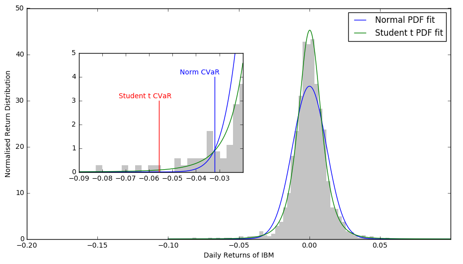
If on the next day ($h=1$) IBM loses more than 1-day VaR (to be between $2.79$% and $3.20$%) how far the actual loss may go? Because Student $t$ distribution applied to the IBM data models the left tail more accurately than the Normal pdf, the value of 1-day Student $t$ CVaR of $5.58$% (red marker in the chart) appears more intuitive and expected somehow.
We know that nothing serious happened on the next day but what if, what if…?! With Conditional Value-at-Risk, as a risk manager, you have been warned…
References
Alexander, C., 2008, Market Risk Analysis. Volume IV., John Wiley & Sons Ltd
Jump Deeper
Student t Distributed Linear Value-at-Risk
Recalibrating Expected Shortfall to Match Value-at-Risk for Discrete Distributions
GARCH(p,q) Model and Trade’s Exit Strategy
Does It Make Sense to Use 1-Hour 1% VaR and ES for Bitcoin?
2 comments
Hi Pawel! Thanks so much for writing up this detailed explanation of VaR and CVaR, super informative for me. For the t distribution, do you mean to use sig_norm and mu_norm, or sig_t and mu_t?
VaR_t = np.sqrt((nu-2)/nu) * t.ppf(1-alpha, nu)*sig_norm – h*mu_norm
CVaR_t = -1/alpha * (1-nu)**(-1) * (nu-2+xanu**2) * \
t.pdf(xanu, nu)*sig_norm – h*mu_norm
I compared your formulas to those on Wikipedia page: https://en.wikipedia.org/wiki/Expected_shortfall#cite_note-:1-11
and they don’t quite match. I don’t know what to make of that.
Thanks! Let me check and come back on this to You!