How to Design Intraday Cryptocurrency Trading Model using Bitcoin-based Signals?

With a growing popularity of cryptocurrencies and their increasing year-over-year traded volumes, crypto algo-trading is a next big thing! If you study this market closely you will notice that it offers quick gains in much shorter unit of time comparing to stocks or FX. No wonder why a participation in trading, even using mobile apps like Coinbase or Binance attracts more people now than ever.

A long-term, systematic winning in crypto-universe is as difficult as in any other trading markets. The risk levels are significantly higher and an intraday volatility can dangerously reduce your position within few minutes! But that’s the beauty in its purest form. This is why it’s worth to sit down and think about some strategies allowing to attack this hostile territory for faint-hearted people.

A quite unique feature of a larger number of traded cryptocurrencies is its noticeable high linear correlation. The co-movements in prices up or down happen nearly instantly within 1-minute long timeframes to the degree you could think of an invisible man pulling all strings at the same time behind the scene. So weird but also so cool! However, where does it all start? Which cryptocurrency is a leading one? Is it a Bitcoin which spreads new buy/sell signals across all crypto-markets and triggers other coins’ prices to rise or fall as a feedback? Partially it’s true. I believe that for many reasons inter alia historical, statutory, or liquidity-related the Bitcoin is the coin all markets’ participants watch very closely. Do they follow it? For sure quantitatively you can easily determine that but finding those coins performing better than Bitcoin over the same period would be a real game changer!

In this post we will design the fundamentals of an algo-trading long model. We will use Bitcoin intraday prices (1-minute OHLC time-series) to identify sudden positive price changes as appealing triggers. Based on them we will simulate trading, i.e. opening a new long position a minute after the trigger and apply 2-step-verification stop-loss for closing our trades. We will assume a fix amount of dollars invested in each open trade and no trading fees for testing core model’s backbone.

1. Collecting 1-Min OHLC Time-Series of Cryptocurrencies

In order to start building a prototype of an algo-trading model we need data. Here I will use 1-min time-series collected for a number of crypto-coins traded versus USD across Coinbase market. The function responsible for fetching the data, ccrypto.getCryptoSeries, will be soon available with a release of my new book Cryptocurrencies with Python. As usual we begin with the import of required Python libraries utilised in today’s code:

# How to Design Intraday Algo-Trading Model for Cryptocurrencies 
# using Bitcoin-based Signals?
# 
# (c) 2020 QuantAtRisk.com, by Pawel Lachowicz

import ccrypto as cc

import numpy as np
import pandas as pd
import matplotlib.dates as mdates
import matplotlib.pyplot as plt
import plotly.graph_objects as go  # good for candlestick charts
import pickle  # for storing Python's dictionaries in a file

import warnings
warnings.filterwarnings("ignore")

# matplotlib color codes
blue, orange, red, green = '#1f77b4', '#ff7f0e', '#d62728', '#2ca02c'
grey8 = (.8,.8,.8)

By employing Python’s dictionaries one can efficiently store many time-series even as pandas’ DataFrame object! If you are new to Python, take a note of it. It’s pretty handy solution I like to use frequently:

# coin selection
coins = ['BTC', 'ETH', 'XRP', 'BCH', 'LTC', 'EOS', 'XTZ', 'LINK', 
         'XLM', 'DASH', 'ETC', 'ATOM']

database = {}
for coin in coins:
    print(coin + '...', end=" ")
    try:
        database[coin] = cc.getCryptoSeries(coin, freq='m', ohlc=True, exch='Coinbase')
        print('downloaded')
    except:
        print('unsuccessful')
    
# save dictionoary with time-series in a file (binary)
with open('timeseries_20200420_20200427.db', 'wb') as handle:
    pickle.dump(database, handle)

BTC... downloaded
ETH... downloaded
XRP... downloaded
BCH... downloaded
LTC... downloaded
EOS... downloaded
XTZ... downloaded
LINK... downloaded
XLM... downloaded
DASH... downloaded
ETC... downloaded
ATOM... downloaded

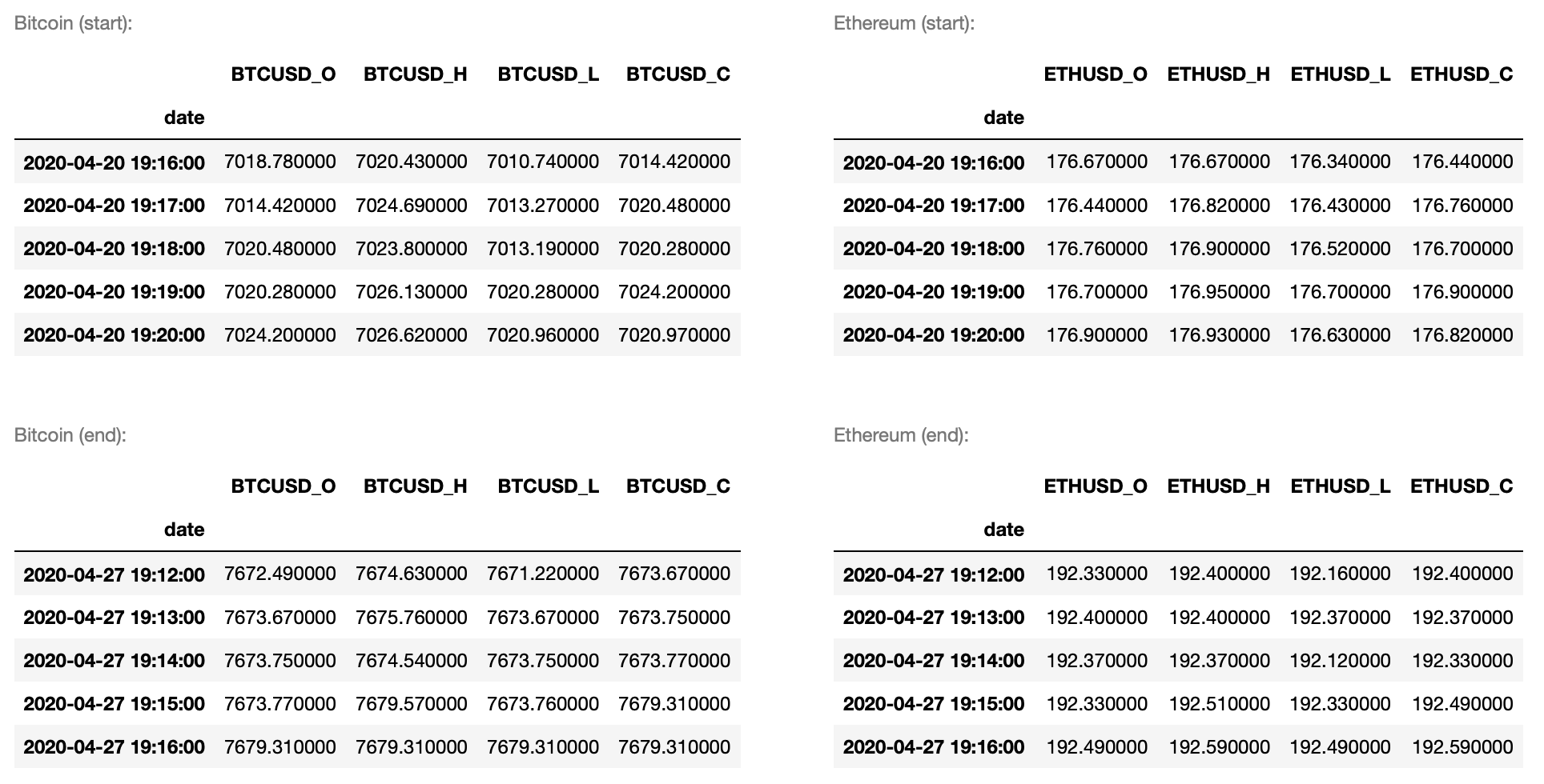
In the above example we target a download of Bitcoin, Ethereum, XRP, Bitcoin Cash, Litecoin, EOS, Tezos, Chainlink, Stellar Lumens, Dash, Ethereum Classic, and Cosmos, respectively. The data will cover the last 7 trading days, i.e. from 2020-Apr-20 till 2020-04-27, in this example. It may happen that for less liquid coins, the time-series will have a number of missing data points. C’est la vie! However, within this research they absence will not be a problem as you will see.

Importing all time-series from the file you can execute by running:

# load time-series from database
with open('timeseries_20200420_20200427.db', 'rb') as handle:
    ts = pickle.load(handle)
    
print(ts.keys())  # get the keys of available time-series

dict_keys(['BTC', 'ETH', 'XRP', 'BCH', 'LTC', 'EOS', 'XTZ', 'LINK', 'XLM', 'DASH', 
           'ETC', 'ATOM'])

or check visually, for instance:

>
cc.displayS([ts['BTC'].head(), ts['ETH'].head()], ['Bitcoin (start)','Ethereum (start)'])
cc.displayS([ts['BTC'].tail(), ts['ETH'].tail()], ['Bitcoin (end)','Ethereum (end)'])

2. From Observations to Triggers

There is no shame to design a model which would open a new position triggered by an event. I am aware that very slowly we are entering a new era in algo-trading to be dominated by artificial intelligence (AI) using more and more frequently machine or deep learning algorithms. Nevertheless, with deeper powers come less transparency. Therefore, dare to know what sort of actions are taken based on what kind of observations made.

In our case, the analysis of many cryptocurrencies traded over the past few months led to a peculiar observation. Namely, if the price of BTC rises quickly up within 1 to 15 minutes, a large number of coins experience a parallel increase in their prices, too.

For technical traders looking at 15-min candlestick chart, the vertical bar builds up on the screen providing them with a strong buy signal (open long position). However, 15 min is a long time in crypto algo-trading…

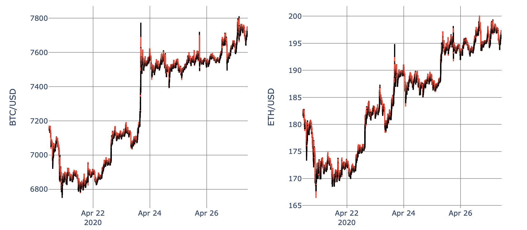
Let’s analyse our data to illustrate what we are talking about by comparing BTC and ETH time-series using plotly library for Python. Plotly offers pretty easy way to visualise the OHLC time-series using candlesticks. The following code does the job for BTC but you can rerun it for any other time-series which we stored in our initial database file (see code lines #40-41).

# candlestick chart for OHLC time-series available as pandas' DataFrames
# employing plotly

# color codes for plotly
whiteP, blackP, redP, greyP = '#FFFFFF', '#000000', '#FF4136', 'rgb(150,150,150)'

fig = go.Figure(data=go.Candlestick(x     = ts['BTC'].index, 
                                    open  = ts['BTC'].iloc[:,0], 
                                    high  = ts['BTC'].iloc[:,1],
                                    low   = ts['BTC'].iloc[:,2],
                                    close = ts['BTC'].iloc[:,3],)
               )
fig.update(layout_xaxis_rangeslider_visible=False)
fig.update_layout(plot_bgcolor=whiteP, width=500)
fig.update_xaxes(showgrid=True, gridwidth=1, gridcolor=greyP)
fig.update_yaxes(showgrid=True, gridwidth=1, gridcolor=greyP)
fig.update_yaxes(title_text='BTC/USD')

# update line and fill colors
cs = fig.data[0]
cs.increasing.fillcolor, cs.increasing.line.color = blackP, blackP
cs.decreasing.fillcolor, cs.decreasing.line.color = redP, redP

fig.show()

For Bitcoin and Ethereum, their 1-min trading patterns display lots of similarities with some prominent tight co-movements:

Here, you can easily spot a spike in Bitcoin price at 16:22 (Apr 23, 2020) and at the same time the corresponding spike in ETH trading:

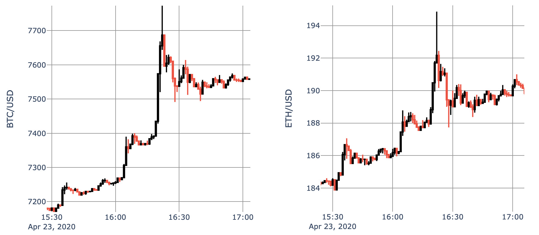
The BTC price moved from the resistance level of 7400 USD up at ca. 7700 USD, i.e. gaining 4% just in 4 minutes! Funny enough, if you compare candle by candle all individual 1-min bars, you will discover a degree how closely both cryptocurrency are traded. The only difference between the two is dictated by traded volume and its expression in price.

3. Triggers to Open Long Position

The examples like the one discussed above there are many more every week! You can convince yourself about that by starting your own data collection/analysis over the upcoming weeks and months. Nothing dramatically won’t change in this matter. Trust me on that.

Within my research I determined that a 0.5% rate of change between BTC close-price “now” and one minute ago can be a good trigger for opening a new trade (long position) at the open-price in next minute.

Since our triggers are Bitcoin-based only, we can determine them working with a local DataFrame btc for a while. Study the code:

btc = ts['BTC']  # assign BTC data to a new temporary variable

btc = btc[['BTCUSD_O', 'BTCUSD_C']]  # limit to Open and Close series

# add a new column with Close price 1 min ago
btc['BTCUSD_C_LAG1'] = btc['BTCUSD_C'].shift(1)

# define a supporting function
def rr(z):
    '''Calculates rate of return [percent].
       Works with two DataFrame's columns as an input.
    '''
    x, y = z[0], z[1]
    return 100*(x/y-1)


# calculate rate of return between:
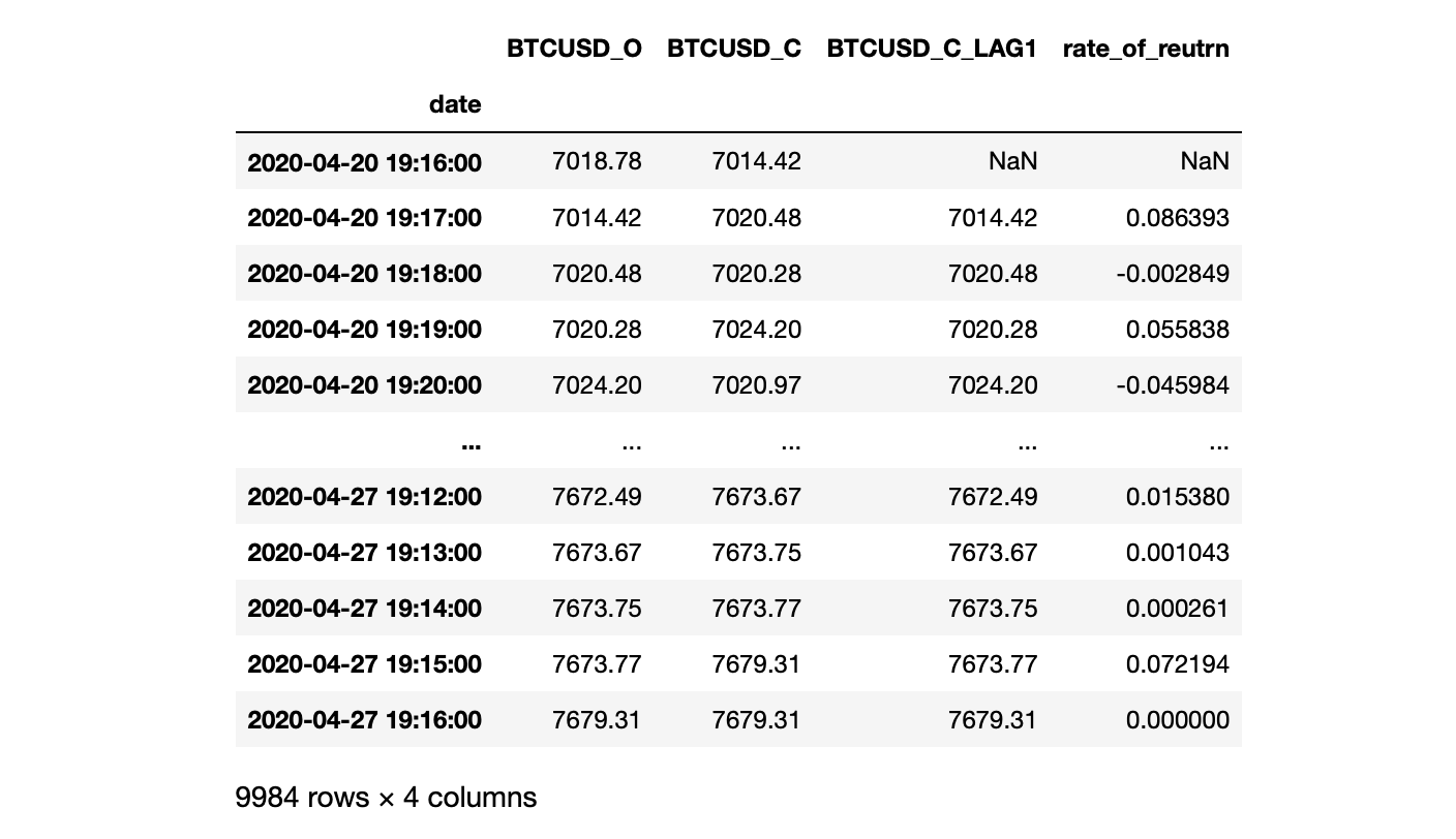
btc['rate_of_reutrn'] = btc[['BTCUSD_C', 'BTCUSD_C_LAG1']].apply(rr, axis=1)

display(btc)

# get rid of NaN rows
btc = btc.dropna()

Assuming $0.5%$ as a threshold, we can find and illustrate all possible triggers as follows:

# select a threshold for triggers
thr = 0.5  # 1-min rate of return greater than 'thr' percent

tmp = btc[btc.rate_of_reutrn > thr]

fig, ax = plt.subplots(1,1,figsize=(15,5))
ax.plot((btc.BTCUSD_C), color=grey8)
ax.plot([tmp.index, tmp.index], [tmp.BTCUSD_O, tmp.BTCUSD_C], color=red)
ax.grid()
ax.legend(['BTCUSD Close Price', 'Triggers'])
plt.gcf().autofmt_xdate()
myFmt = mdates.DateFormatter('%Y-%m-%d %H:%M')
plt.gca().xaxis.set_major_formatter(myFmt)

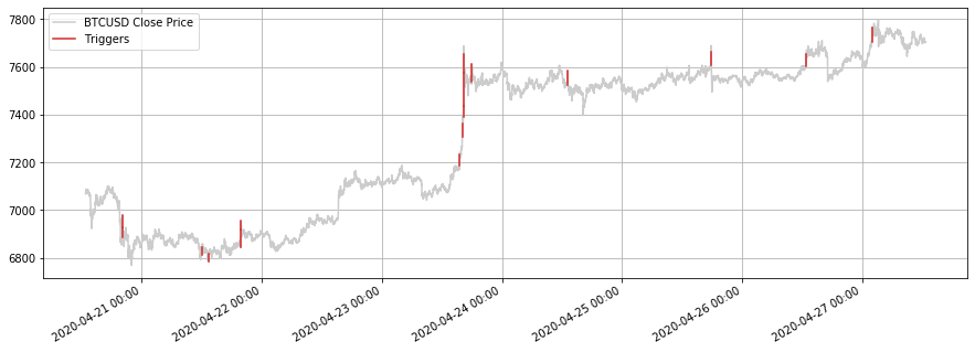
Great. The number of potential triggers for a considered time-series span is low (16). The triggers are determined at:

print(tmp.index)

DatetimeIndex(['2020-04-20 20:05:00', '2020-04-20 20:06:00',
               '2020-04-21 11:59:00', '2020-04-21 13:23:00',
               '2020-04-21 19:50:00', '2020-04-21 19:51:00',
               '2020-04-23 15:35:00', '2020-04-23 16:05:00',
               '2020-04-23 16:19:00', '2020-04-23 16:20:00',
               '2020-04-23 16:21:00', '2020-04-23 18:00:00',
               '2020-04-24 13:05:00', '2020-04-25 17:50:00',
               '2020-04-26 12:49:00', '2020-04-27 02:00:00'],
              dtype='datetime64[ns]', name='date', freq=None)

which mean, according to our “simulated” trading strategy, we will open a new trade at an open-price at:

# time index when a new position will be opened
ind_buy = tmp.index + pd.Timedelta(minutes = 1)
print(ind_buy)

DatetimeIndex(['2020-04-20 20:06:00', '2020-04-20 20:07:00',
               '2020-04-21 12:00:00', '2020-04-21 13:24:00',
               '2020-04-21 19:51:00', '2020-04-21 19:52:00',
               '2020-04-23 15:36:00', '2020-04-23 16:06:00',
               '2020-04-23 16:20:00', '2020-04-23 16:21:00',
               '2020-04-23 16:22:00', '2020-04-23 18:01:00',
               '2020-04-24 13:06:00', '2020-04-25 17:51:00',
               '2020-04-26 12:50:00', '2020-04-27 02:01:00'],
              dtype='datetime64[ns]', name='date', freq=None)

4. 2-Step Verification of Stop Loss as a Trigger to Close Long Position

There are hundreds of ways to close your open trade. Here, let me apply a simple stop loss method. It may be activated in two instances: (1) if the rolling PnL of the trade falls below certain threshold (thr1), or (2) if the drawdown calculated as a relative difference between the rolling maximal trade’s PnL and the current trade’s PnL exceeds a certain level (thr2):

def check_stoploss(z, thr1=-0.15, thr2=-0.15):
    p1, p2 = z
    if p1 < thr1 or p2 < thr2:
        return False  # close position
    else:
        return True  # hold position open

Above, both threshold were assumed to be $-15%$. In other words, in the trade’s PnL will drop below $-15%$ (thr1) we will close position at the closest close price. Also, say, it the trade’s PnL will rise by $31%$ to a new maximum, and since that moment the price will drop by more than $-15%$ (thr2), we will cash in (hopefully with a positive PnL of that trade).

5. Simulated Trading and Trade Tracking

5.1. Bitcoin as a Benchmark

Given the rules when to open and when to close each trade, in the following simulation of intraday algo-trading, let’s assume we invest every time 1000 USD in each trade (again, no fee structure applied here). To begin, we can analyse what-if we were trading Bitcoin only. Our code is a loop over all pre-determined 16 triggers. It is written in a way to gather information on rolling trade’s PnL, maximal PnL reached/updated, and rolling trade’s PnL drawdown supplemented with a nice visualisation:

backtested_coins = ['BTC']

results = {}

for coin in backtested_coins:

    # read OHLC price time-series
    df = ts[coin]

    tradePnLs = list()

    for ib in range(len(ind_buy)):
        i = ind_buy[ib]
        try:
            op = df.loc[i][0]

            # Trade No. 'ib' DataFrame
            tmp = df[df.index >= i]
            tmp['open_price'] = op  # trade's open price
            tmp['current_price'] = df[coin + 'USD_C']
            tmp['pnl'] = tmp.current_price / op - 1

            fi = True
            out1 = list()
            out2 = list()
            for j in range(tmp.shape[0]):
                if fi:
                    maxPnL = tmp.pnl[j]
                    maxClose = tmp.iloc[j, 3]
                    fi = False
                else:
                    if tmp.pnl[j] > maxPnL:
                        maxPnL = tmp.pnl[j]
                        maxClose = tmp.iloc[j, 3]
                out1.append(maxPnL)
                out2.append(maxClose)  # close price

            tmp['maxPnL'] = out1
            tmp['maxClose'] = out2
            tmp['drawdown'] = tmp.current_price / tmp.maxClose - 1
            tmp['hold'] = tmp[['pnl', 'drawdown']].apply(check_stoploss, axis=1)

            # execute selling if detected
            sell_executed = True
            try:
                sell_df = tmp[tmp.hold == 0]
                sell_time, close_price = sell_df.index[0], sell_df.current_price[0]
                tmpT = tmp[tmp.index <= sell_time]
            except:
                sell_executed = False

            #display(tmp.iloc[:,:].head(10))

            plt.figure(figsize=(15,4))
            plt.grid()
            plt.plot(tmp.pnl, color=grey8, label = "Rolling trade's PnL (open trade)")
            if sell_executed:
                plt.plot(tmpT.pnl, color=blue, label = "Rolling trade's PnL (closed)")
                plt.title("Trade's final PnL = %.2f%%" % (100*tmpT.iloc[-1,6]))
                tradePnLs.append(tmpT.iloc[-1,6])
            else:
                plt.title("Current trade's PnL = %.2f%%" % (100*tmp.iloc[-1,6]))
                tradePnLs.append(tmp.iloc[-1,6])
            plt.plot(tmp.maxPnL, color=orange, label = "Rolling maximal trade's PnL")
            plt.plot(tmp.index, np.zeros(len(tmp.index)), '--k')
            plt.suptitle('Trade No. %g opened %s @ %.2f USD' % (ib+1, i, df.loc[i][0]))
            plt.legend()
            locs, labels = plt.xticks()
            plt.xticks(locs, [len(list(labels))*""])
            plt.show()

            plt.figure(figsize=(14.85,1.5))
            plt.grid()
            plt.plot(tmp.drawdown, color=red, label = "Rolling trade's drawdown")
            plt.plot(tmp.index, np.zeros(len(tmp.index)), '--k')
            plt.gcf().autofmt_xdate()
            myFmt = mdates.DateFormatter('%Y-%m-%d %H:%M')
            plt.gca().xaxis.set_major_formatter(myFmt)
            plt.legend()
            plt.show()

            print("nn")
        except:
            pass

For the first trade from our list, keeping stop loss configuration at thr1=-0.15 and thr2=-0.15 level, we get:

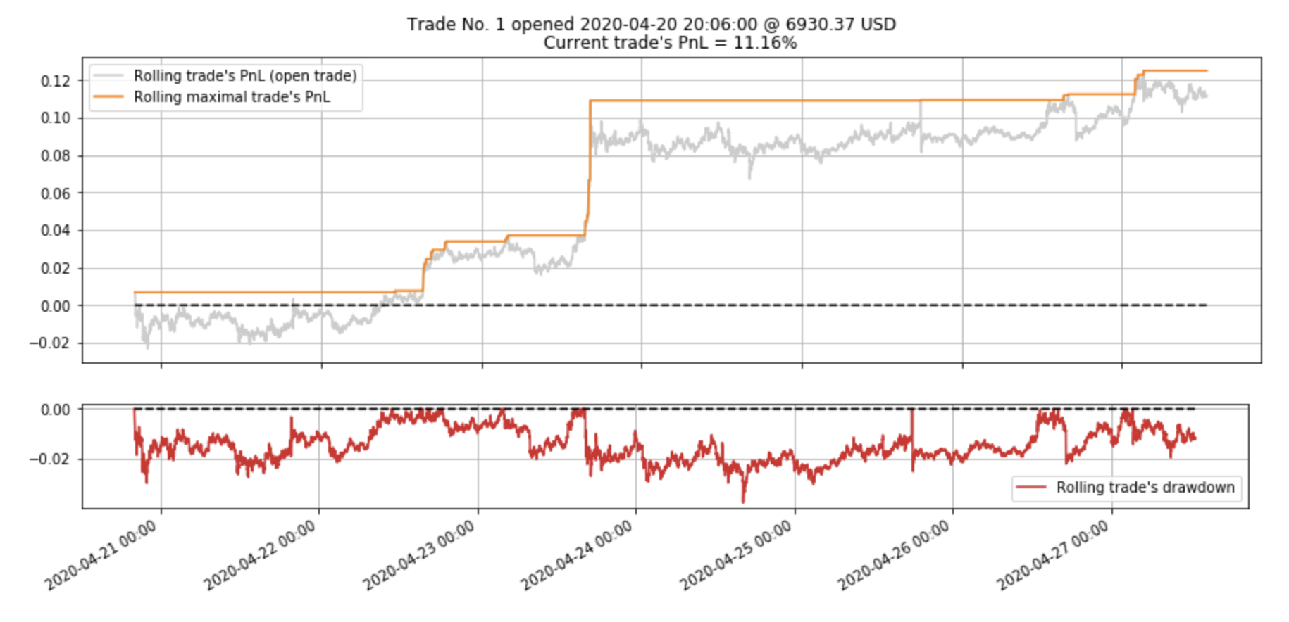
what simply can be understood as a trade still open earning $+11.16%$ (at the end of time-series). No stop loss has been triggered this time.

However, if we allow to set thr2=-0.03 the trade will be automatically closed by the execution of stop-loss process if its PnL falls more than $3%$ from the maximal value of the PnL reached by the trade since its opening:

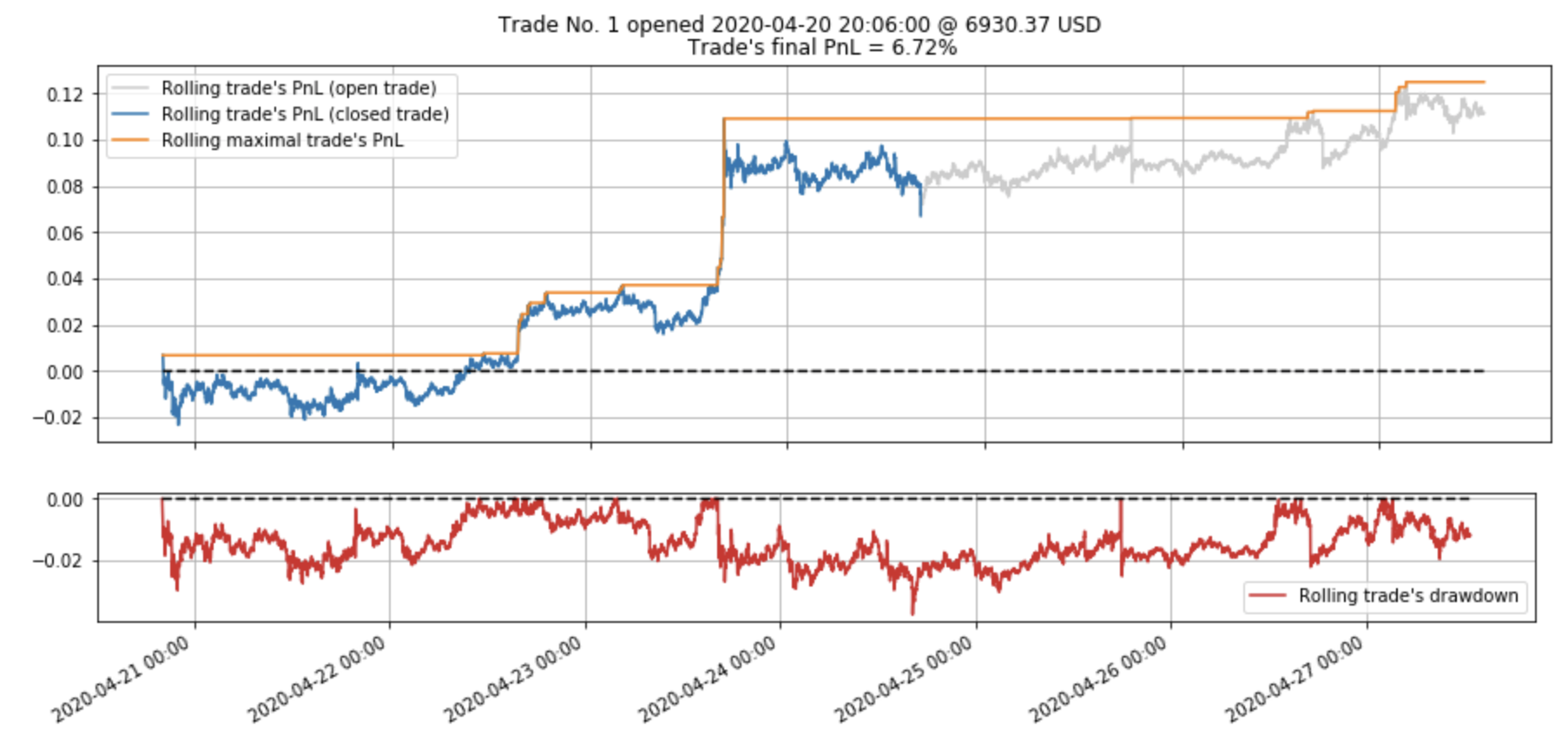
In this case we cash in $+6.72%$ on our investment or $+67.20$ USD.

I hope that with this example you can understand the code of simulated trading (trade by trade) better. Of course, this solely presents one of many ways how one can “take care” of your trades during live trading. My purpose here was to provide you with an intuitive illustration on possibility to design and backtest your own trading strategy given a set of reliable time-series.

If we supplement a loop above with the code that follows, we will be able to prepare a trading-log. If the trades were closed due to stop loss, you would read the trade’s PnL as realised PnL while in all other cases as unrealised PnL:

    c = 1000  # initial investment (fixed; per each trade)
    tradePnLs = np.array(tradePnLs)
    n_trades = len(tradePnLs)
    res = pd.DataFrame(tradePnLs, columns=['Trade_PnL'])
    res['Investment_USD'] = c
    res['Trade_ROI_USD'] = np.round(c * (tradePnLs + 1),2)
    res.index = np.arange(1,n_trades+1)
    res.index.name = 'Trade_No'
    ROI = res.Trade_ROI_USD.sum() - (n_trades * c)
    ROI_pct = 100 * (res.Trade_ROI_USD.sum() / (n_trades * c) - 1)
    tot_pnl = res.Trade_ROI_USD.sum()
    res.loc[res.shape[0]+1] = ['', np.round(n_trades * c,2), '']
    res.rename(index = {res.index[-1] : "Total Investment (USD)"}, inplace=True)
    res.loc[res.shape[0]+1] = ['', '', np.round(tot_pnl,2)]
    res.rename(index = {res.index[-1] : "Total PnL (USD)"}, inplace=True)
    res.loc[res.shape[0]+1] = ['', '', np.round(ROI,2)]
    res.rename(index = {res.index[-1] : "Total ROI (USD)"}, inplace=True)
    res.loc[res.shape[0]+1] = ['', '', np.round(ROI_pct,2)]
    res.rename(index = {res.index[-1] : "Total ROI (%)"}, inplace=True)
    
    results[coin] = res

In case of BTC we obtain:

display(results['BTC'])

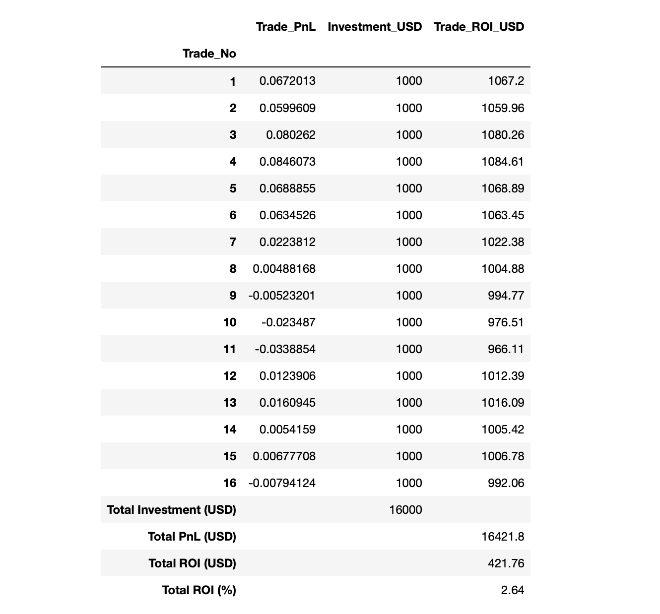
After 7 days of running this strategy $+2.64%$ gain seems to be low. It’s not if you put ten time more on the table instead of 16,000 USD. Let’s check whether we can beat that benchmark using the same set of Bitcoin-based triggers in trading other cryptocurrencies over the same time period.

5.2. ETH, XTZ, DASH, and LINK vs Benchmark

Without any further delay, replace a current code line #127 with the following set:

backtested_coins = ['BTC', 'ETH', 'XTZ', 'DASH', 'LINK']

and re-run the entire simulation. Based on the analysis of the outcomes:

cc.displayS([results['ETH'], results['XTZ']], ['Trading ETH/USD', 'Trading XTZ/USD'])
cc.displayS([results['DASH'], results['LINK']],['Trading DASH/USD', 'Trading LINK/USD'])

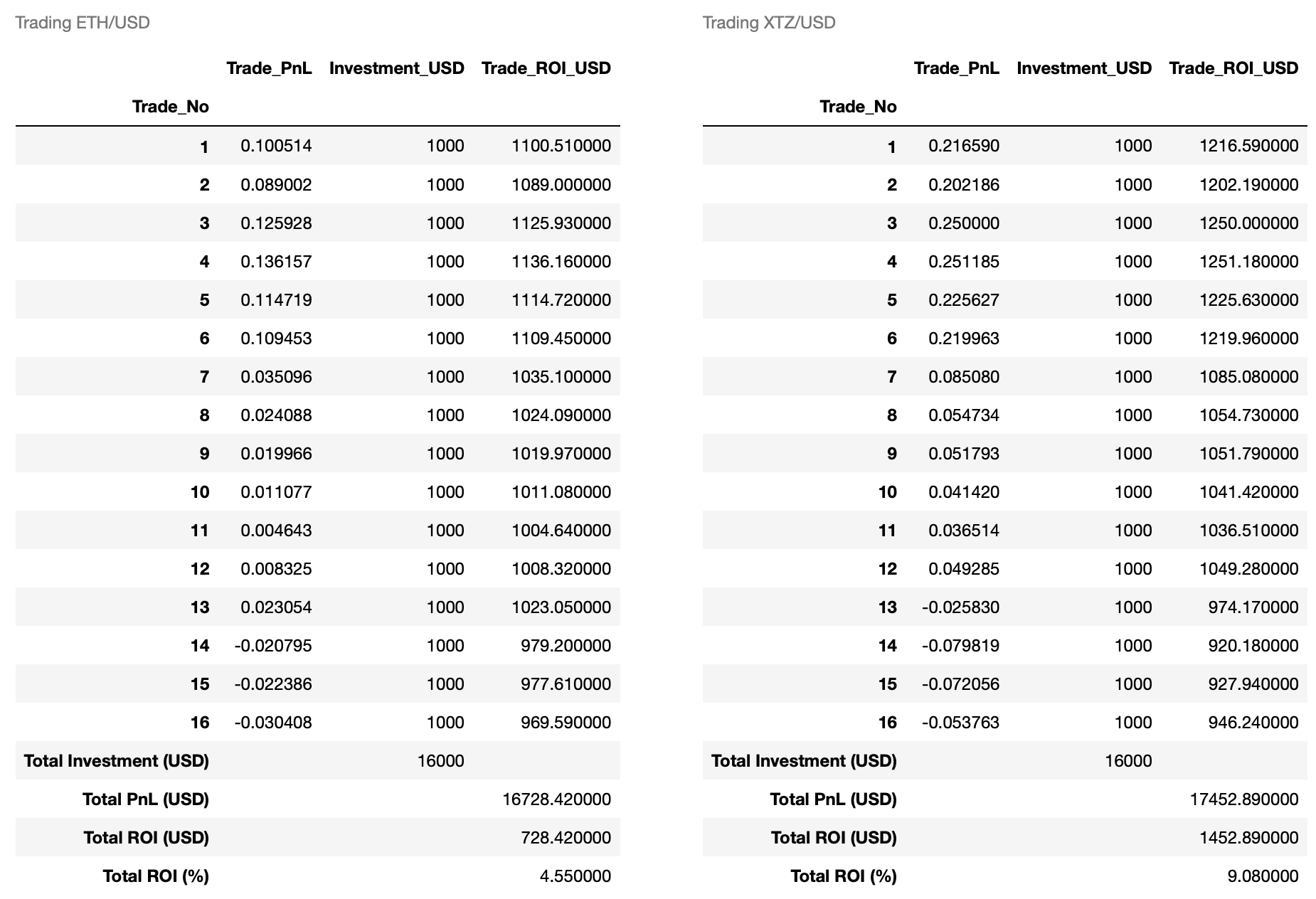
A clear winner is Tezos (XTZ) with the best results of $+25.12%$ profit in a single trade.

6. Summary

In this post we have learnt how to approach intraday trading data and design algo-trading strategy based on live events (triggers). The potential for big gains in short time is huge but before you retire early, you have to come up with a good trading model. At the very beginning I told you that a long-term, systematic winning in crypto-universe is as difficult as in any other trading markets. Hopefully, the lesson taken from this article you can easily leverage to your benefits. Happy trading!

DOWNLOADABLES:
timeseries_20200420_20200427.db (3.39 MB)