Black Swans and Extreme Loss Modeling

When I read the book of Nassim Nicholas Taleb Black Swan my mind was captured by the beauty of extremely rare events and, concurrently, devastated by the message the book sent: the non-computability of the probability of the consequential rare events using scientific methods (as owed to the very nature of small probabilities). I rushed to the local library to find out what had been written on the subject. Surprisingly I discovered the book of Embrechts, Kluppelberg & Mikosh on Modelling Extremal Events for Insurance and Finance which appeared to me very inaccessible, loaded with heavy mathematical theorems and proofs, and a negligible number of practical examples. I left it on the shelf to dust for a longer while until last week when a fresh drive to decompose the problem came back to me again.

In this article I will try to take you for a short but efficient journey through the part of the classical extreme value theory, namely, fluctuations of maxima, and fulfil the story with easy-to-follow procedures on how one may run simulations of the occurrences of extreme rare losses in financial return series. Having this experience, I will discuss briefly the inclusion of resulting modeling to the future stock returns.

1. The Theory of Fluctuations of Maxima

Let’s imagine we have a rich historical data (time-series) of returns for a specific financial asset or portfolio of assets. A good and easy example is the daily rate of returns, $R_i$, for a stock traded e.g. at NASDAQ Stock Market,
$$
R_t = \frac{P_t}{P_{t-1}} – 1 \ ,
$$ where $P_t$ and $P_{t-1}$ denote a stock price on a day $t$ and $t-1$, respectively. The longer time coverage the more valuable information can be extracted. Given the time-series of daily stock returns, $\{R_i\}\ (i=1,…,N)$, we can create a histogram, i.e. the distribution of returns. By the rare event or, more precisely here, the rare loss we will refer to the returns placed in the far left tail of the distribution. As an assumption we also agree to $R_1,R_2,…$ to be the sequence of iid non-degenerate rvs (random variables) with a common df $F$ (distribution function of $F$). We define the fluctuations of the sample maxima as:
$$
M_1 = R_1, \ \ \ M_n = \max(R_1,…,R_n) \ \mbox{for}\ \ n\ge 2 \ .
$$ That simply says that for any time-series $\{R_i\}$, there is one maximum corresponding to the rv (random variable) with the most extreme value. Since the main line of this post is the investigation of maximum losses in return time-series, we are eligible to think about negative value (losses) in terms of maxima (therefore conduct the theoretical understanding) thanks to the identity:
$$
\min(R_1,…,R_n) = -\max(-R_1,…,-R_n) \ .
$$ The distribution function of maximum $M_n$ is given as:
$$
P(M_n\le x) = P(R_1\le x, …, R_n\le x) = P(R_1\le x)\cdots P(R_n\le x) = F^n(x)
$$ for $x\in\Re$ and $n\in\mbox{N}$.

What the extreme value theory first ‘investigates’ are the limit laws for the maxima $M_n$. The important question here emerges: is there somewhere out there any distribution which satisfies for all $n\ge 2$ the identity in law
$$
\max(R_1,…,R_n) = c_nR + d_n
$$ for appropriate constants $c_n>0$ and $d_n\in\Re$, or simply speaking, which classes of distributions $F$ are closed for maxima? The theory defines next the max-stable distribution within which a random variable $R$ is called max-stable if it satisfies a aforegoing relation for idd $R_1,…,R_n$. If we assume that $\{R_i\}$ is the sequence of idd max-stable rvs then:
$$
R = c_n^{-1}(M_n-d_n)
$$ and one can say that every max-stable distribution is a limit distribution for maxima of idd rvs. That brings us to the fundamental Fisher-Trippett theorem saying that if there exist constants $c_n>0$ and $d_n\in\Re$ such that:
$$
c_n^{-1}(M_n-d_n) \rightarrow H, \ \ n\rightarrow\infty\ ,
$$ then $H$ must be of the type of one of the three so-called standard extreme value distributions, namely: Fréchet, Weibull, and Gumbel. In this post we will be only considering the Gumbel distribution $G$ of the corresponding probability density function (pdf) $g$ given as:
$$
G(z;\ a,b) = e^{-e^{-z}} \ \ \mbox{for}\ \ z=\frac{x-b}{a}, \ x\in\Re
$$ and
$$
g(z;\ a,b) = b^{-1} e^{-z}e^{-e^{-z}} \ .
$$ where $a$ and $b$ are the location parameter and scale parameter, respectively. Having defined the extreme value distribution and being now equipped with a better understanding of theory, we are ready for a test drive over daily roads of profits and losses in the trading markets. This is the moment which separates men from boys.

2. Gumbel Extreme Value Distribution for S&P500 Universe

As usual, we start with entrée. Our goal is to find the empirical distribution of maxima (i.e. maximal daily losses) for all stocks belonging to the S&P500 universe between 3-Jan-1984 and 8-Mar-2011. There were $K=954$ stocks traded within this period and their data can be downloaded here as a sp500u.zip file (23.8 MB). The full list of stocks’ names is provided in sp500u.lst file. Therefore, performing the data processing in Matlab, first we need to compute a vector storing daily returns for each stock, and next find the corresponding minimal value $M_n$ where $n$ stands for the length of each return vector:

% Black Swan and Extreme Loss Modeling
%  using Gumbel distribution and S&P500 universe
%
% (c) 2013 QuantAtRisk, by Pawel Lachowicz


clear all; close all; clc;
tic;

%% DATA READING AND PREPROCESSING

% read a list of stock names
StockNames=dataread('file',['sp500u.lst'],'%s','delimiter', '\n');
K=length(StockNames); % the number of stocks in the universe
% path to data files
path=['./SP500u'];

fprintf('data reading and preprocessing..\n');
for si=1:K
    % --stock name
    stock=StockNames{si};
    fprintf('%4.0f  %7s\n',si,stock);
    % --load data
    n=[path,'/',stock,'.dat'];
    % check for NULL and change to NaN (using 'sed' command
    % in Unix/Linux/MacOS environment)
    cmd=['sed -i ''s/NULL/NaN/g''',' ',n]; [status,result]=system(cmd);
    % construct FTS object for daily data
    FTS=ascii2fts(n,1,2);
    % fill any missing values denoted by NaNs
    FTS=fillts(FTS);
    % extract the close price of the stock
    cp=fts2mat(FTS.CLOSE,0);
    % calculate a vector with daily stock returns and store it in
    % the cell array
    R{si}=cp(2:end)./cp(1:end-1)-1;
end

%% ANALYSIS

% find the minimum daily return value for each stock
Rmin=[];
for si=1:K
    Mn=min(R{si},[],1);
    Rmin=[Rmin; Mn];
end

Having that ready, we fit the data with the Gumbel function which (as we believe) would describe the distribution of maximal losses in the S&P500 universe best:

% fit the empirical distribution with Gumbel distribution and 
% estimate the location, a, and scale, b, parameter
[par,parci]=evfit(Rmin);
a=par(1); 
b=par(2);

% plot the distribution
x=-1:0.01:1;
hist(Rmin,-1:0.01:0);
h=findobj(gca,'Type','patch');
set(h,'FaceColor',[0.7 0.7 0.7],'EdgeColor',[0.6 0.6 0.6]);
h=findobj(gca,'Type','box');
set(h,'Color','k');

% add a plot of Gumbel pdf 
pdf1=evpdf(x,a,b);
y=0.01*length(Rmin)*pdf1;
line(x,y,'color','r'); box on;
xlabel('R_{min}');
ylabel(['f(R_{min}|a,b)']);
text(-1,140,['a = ',num2str(paramEstsMinima(1),3)]);
text(-1,130,['b = ',num2str(paramEstsMinima(2),3)]); 
xlim([-1 0]);

The maximum likelihood estimates of the parameters $a$ and $b$ and corresponding 95% confidence intervals we can find as follows:

>> [par,parci]=evfit(Rmin)

par =
   -0.2265    0.1135

parci =
   -0.2340    0.1076
   -0.2190    0.1197

That brings us to a visual representation of our analysis:

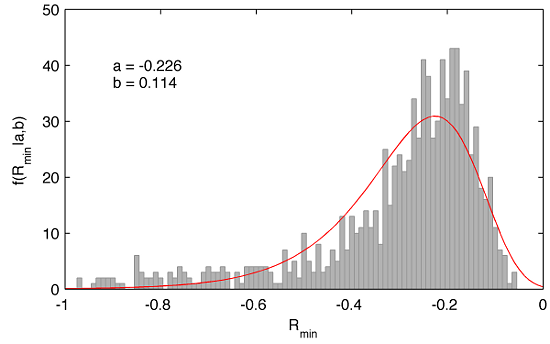
This is a very important result communicating that the expected value of extreme daily loss is equal about -22.6%. However, the left tail of the fitted Gumbel distribution extends far up to nearly -98% although the probability of the occurrence of such a massive daily loss is rather low.

On the other hand, the expected value of -22.6% is surprisingly close to the trading down-movements in the markets on Oct 19, 1987 known as Black Monday when Dow Jones Industrial Average (DJIA) dropped by 508 points to 1738.74, i.e. by 22.61%!

3. Blending Extreme Loss Model with Daily Returns of a Stock

Probably you wonder how can we include the results coming from the Gumbel modeling for the prediction of rare losses in the future daily returns of a particular stock. This can be pretty straightforwardly done combining the best fitted model (pdf) for extreme losses with stock’s pdf. To do it properly we need to employ the concept of the mixture distributions. Michael B. Miller in his book Mathematics and Statistics for Financial Risk Management provides with a clear idea of this procedure. In our case, the mixture density function $f(x)$ could be denoted as:
$$
f(x) = w_1 g(x) + (1-w_1) n(x)
$$ where $g(x)$ is the Gumbel pdf, $n(x)$ represents fitted stock pdf, and $w_1$ marks the weight (influence) of $g(x)$ into resulting overall pdf.

In order to illustrate this process, let’s select one stock from our S&P500 universe, say Apple Inc. (NASDAQ: AAPL), and fit its daily returns with a normal distribution:

% AAPL daily returns (3-Jan-1984 to 11-Mar-2011)
rs=R{18};
figure(2);
hist(rs,50);
h=findobj(gca,'Type','patch');
set(h,'FaceColor',[0.7 0.7 0.7],'EdgeColor',[0.6 0.6 0.6]);
h=findobj(gca,'Type','box');
set(h,'Color','k');
% fit the normal distribution and plot the fit
[muhat,sigmahat]=normfit(rs)
x =-1:0.01:1;
pdf2=normpdf(x,muhat,sigmahat);
y=0.01*length(rs)*pdf2;
hold on; line(x,y,'color','r');
xlim([-0.2 0.2]); ylim([0 2100]);
xlabel('R');

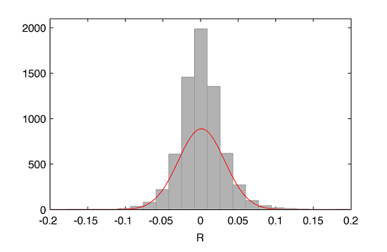
where the red line represents the fit with a mean of $\mu=0.0012$ and a standard deviation $\sigma=0.0308$.

We can obtain the mixture distribution $f(x)$ executing a few more lines of code:

% Mixture Distribution Plot
figure(3);
w1= % enter your favorite value, e.g. 0.001
w2=1-w1;
pdfmix=w1*(pdf1*0.01)+w2*(pdf2*0.01);  % note: sum(pdfmix)=1 as expected
x=-1:0.01:1;
plot(x,pdfmix);
xlim([-0.6 0.6]);

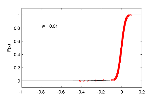
It is important to note that our modeling is based on $w_1$ parameter. It can be intuitively understood as follows. Let’s say that we choose $w_1=0.01$. That would mean that Gumbel pdf contributes to the overall pdf in 1%. In the following section we will see that if a random variable is drawn from the distribution given by $f(x)$, $w_1=0.01$ simply means (not exactly but with a sufficient approximation) that there is 99% of chances of drawing this variable from $n(x)$ and only 1% from $g(x)$. The dependence of $f(x)$ on $w_1$ illustrates the next figure:

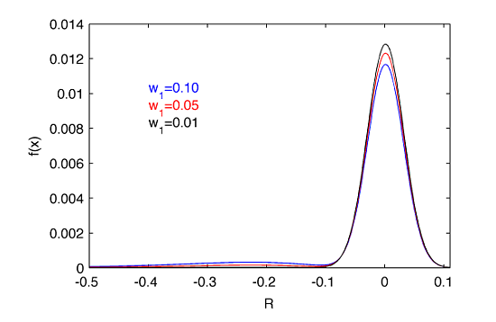
It is well visible that a selection of $w_1>0.01$ would be a significant contributor to the left tail making it fat. This is not the case what is observed in the empirical distribution of daily returns for AAPL (and in general for majority of stocks), therefore we rather expect $w_1$ to be much much smaller than 1%.

4. Drawing Random Variables from Mixture Distribution

A short break between entrée and main course we fill with a sip of red wine. Having discrete form of $f(x)$ we would like to be able to draw a random variable from this distribution. Again, this is easy too. Following a general recipe, for instance given in the Chapter 12.2.2 of Philippe Jorion’s book Value at Risk: The New Benchmark for Managing Financial Risk, we wish to use the concept of inverse transform method. In first step we use the output (a random variable) coming from a pseudo-random generator drawing its rvs based on the uniform distribution $U(x)$. This rv is always between 0 and 1, and in the last step is projected on the cumulative distribution of our interest $F(x)$, what in our case would correspond to the cumulative distribution for $f(x)$ pdf. Finally, we read out the corresponding value on the x-axis: a rv drawn from $f(x)$ pdf. Philippe illustrates that procedure more intuitively:

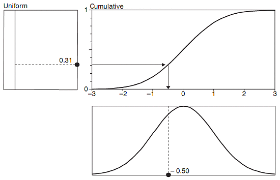
This methods works smoothly when we know the analytical form of $F(x)$. However, if this not in the menu, we need to use a couple of technical skills. First, we calculate $F(x)$ based on $f(x)$. Next, we set a very fine grid for $x$ domain, and we perform interpolation between given data points of $F(x)$.

% find cumulative pdf, F(x)
figure(4);
s=0;
x=-1;
F=[];
for i=1:length(pdfmix);
    s=s+pdfmix(i);
    F=[F; x s];
    x=x+0.01;
end
plot(F(:,1),F(:,2),'k')
xlim([-1 1]); ylim([-0.1 1.1]);
% perform interpolation of cumulative pdf using very fine grid
xi=(-1:0.0000001:1);
yi=interp1(F(:,1),F(:,2),xi,'linear'); % use linear interpolation method
hold on; plot(xi,yi);

The second sort of difficulty is in finding a good match between the rv drawn from the uniform distribution and approximated value for our $F(x)$. That is why a very fine grid is required supplemented with some matching techniques. The following code that I wrote deals with this problem pretty efficiently:

% draw a random variable from f(x) pdf: xi(row)
tF2=round((round(100000*yi')/100000)*100000);
RV=[];
for k=1:(252*40)
    notok=false;
    while(~notok)
        tU=round((round(100000*rand)/100000)*100000);
        [r,c,v]=find(tF2==tU);
        if(~isempty(r))
            notok=true;
        end
    end
    if(length(r)>1)
        rv=round(2+(length(r)-2)*rand);
        row=r(rv); 
    else
        row=r(1);
    end
    % therefore, xi(row) is a number represting a rv
    % drawn from f(x) pdf; we store 252*40 of those
    % new rvs in the following matrix:
    RV=[RV; xi(row) yi(row)];
end
% mark all corresponding rvs on the cumulative pdf
hold on; plot(RV(:,1),RV(:,2),'rx');

Finally, as the main course we get and verify the distribution of a large number of new rvs drawn from $f(x)$ pdf. It is crucial to check whether our generating algorithm provides us with a uniform coverage across the entire $F(x)$ plot,

where, in order to get more reliable (statistically) results, we generate 10080 rvs which correspond to the simulated 1-day stock returns for 252 trading days times 40 years.

5. Black Swan Detection

A -22% collapse in the markets on Oct 19, 1978 served as a day when the name of Black Swan event took its birth or at least had been reinforced in the financial community. Are black swans extremely rare? It depends. If you live for example in Perth, Western Australia, you can see a lot of them wandering around. So what defines the extremely rare loss in the sense of financial event? Let’s assume by the definition that by Black Swan event we will understand of a daily loss of 20% or more. If so, using the procedure described in this post, we are tempted to pass from the main course to dessert.

Our modeling concentrates around finding the most proper contribution of $w_1g(x)$ to resulting $f(x)$ pdf. As an outcome of a few runs of Monte Carlo simulations with different values of $w_1$ we find that for $w_1=[0.0010,0.0005,0.0001]$ we detect in the simulations respectively 9, 5, and 2 events (rvs) displaying a one-day loss of 20% or more.

Therefore, the simulated daily returns for AAPL, assuming $w_1=0.0001$, generate in the distribution two Black Swan events, i.e. one event per 5040 trading days, or one per 20 years:

That result agrees quite well with what has been observed so far, i.e. including Black Monday in 1978 and Flash Crash in intra-day trading on May 6, 2010 for some of the stocks.

Acknowledgements

I am grateful to Peter Urbani from New Zealand for directing my attention towards Gumbel distribution for modeling very rare events.