They say that small fishes buy and sell driven by unstable waters but only big whales make the waves really huge. Recently, this quite popular phrase, makes sense when it comes to cryptocurrency trading influenced by sudden dives of the Bitcoin price. The strategies of buying and selling executed by the whales, often referred to as the institutional buying/selling, may differ in their characteristics but when they sell, they sell fast. This BTC sell-off triggers the sell-offs in other crypto-assets. The correlation is evident in the price charts. But are we misled by an optical illusion?
In this post we will have a quantitative look at this phenomenon. In particular, we will analyse a very recent sell-off of the Bitcoin after it reached U\$61,788 on 2021-03-13 followed by the prices sliding down to U\$54,568 (-11.68%) just two days later according to Coinbase Pro data. Using Python, we will develop a code helping us to calculate a time-dependent fraction of crypto-assets which 1-minute close prices responded exactly the same way as Bitcoin did. This method differs from a classical linear correlation method as the instantaneous price movements are captured instead of long-term relationships among the price points. We demonstrate that the fraction of assets following BTC may be as high as 95% to 100% in certain minutes of trading. We also postulate that a 5-min rolling mean of the computed average instantaneous correlation can be used as a short-term (lagged) sell-off risk measure for crypto-assets.
1. Collecting Suitable Data
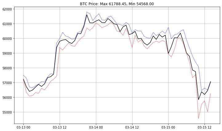
As usual, we make use of data provided by Coinbase exchange. The starting point to the analysis is a current landscape of the Bitcoin trading:
# Introduction to Sell-Off Analysis for Crypto-Assets: Triggered by Bitcoin?
# (c) 2021 QuantAtRisk.com

import ccrypto as cc
import numpy as np
import pandas as pd
import pickle
import matplotlib.pyplot as plt
#from IPython.core.display import display  # for Jupyter Notebooks only

grey  = (.8,.8,.8) # color

# download BTC OHLC prices
b = cc.getCryptoSeries('BTC', 'USD', freq='h', ohlc=True, exch='Coinbase', \
                            start_date='2021-03-13 00:00')

fig, ax1 = plt.subplots(1,1, figsize=(12,7))
ax1.plot(b.BTCUSD_H, 'b:')
ax1.plot(b.BTCUSD_C, 'k')
ax1.plot(b.BTCUSD_L, 'r:')
ax1.grid()
plt.title('BTC Price: Max %.2f, Min %.2f' % (b.BTCUSD_H.max(), b.BTCUSD_L.min()))
Next, let us fetch the close price series for a number of most popular cryptocurrencies at Coinbase for which the 1-min data are available. The reason we wish to have a look at the price movements with 1-min time resolution is to measure as accurately as possible the most direct or indirect feedback of specific crypto-asset price to BTC itself.
We select the universe constructed from the following crypto-assets:
# crypto-currencies
ccys = ['BTC', 'ETH', 'LTC', 'LINK', 'BCH', 'XLM', 'WBTC', 'AAVE', 'EOS', 'ATOM',
        'XTZ', 'DASH', 'GRT', 'MKR', 'SNX', 'ALGO', 'COMP', 'ZEC', 'ETC', 'YFI',
        'CGLD', 'OMG', 'UNI', 'UMA']
In the following part of the code, we will fetch the data and, concurrently, construct a DataFrame. The loop is designed so that first will grab the price-series of BTC/USD and next, within subsequent iterations, we will apply so-called LEFT JOIN. Since the BTC series is a crypto-asset traded for the longest time in a “crypto history”, all other cryptocurrencies in our universe will display shorter periods of overall trading activities, therefore less data points. By the application of, well-known for all SQL users, LEFT JOIN operation (here in Python executed by pd.merge function; see lines #45-46), we simply allow to uses BTC’s index (timestamps) as the baseline, and match others’ coins prices for exisiting indexes.
timeseries = {}  # empty dictionary
fi = True  # first iteration

plt.figure(figsize=(12,7))

# loop over all crypto-assets
for ccy  in ccys:
    # fetch close price time-series with 1-min resolution
    timeseries[ccy] = cc.getCryptoSeries(ccy, 'USD', freq='m', exch='Coinbase', \
                            start_date='2021-03-15 00:00')

    # construct a DataFrame using LEFT JOIN
    if fi:
        df = timeseries[ccy]
        fi = False
    else:
        df = pd.merge(left=df, right=timeseries[ccy], how='left',
                      left_index=True, right_index=True)

    # plot standarised time-series
    plt.plot((timeseries[ccy]-timeseries[ccy].mean())/timeseries[ccy].std(), color=grey)

plt.plot((timeseries['BTC']-timeseries['BTC'].mean())/timeseries['BTC'].std(),
         color='r', label='Bitcoin')
plt.legend(loc=3)
plt.grid()
plt.ylabel('Standardised Price')
plt.xlabel('Date/Time')
plt.savefig("/Users/pawel/Desktop/trig2.png", bbox_inches='tight')
By the way we included plotting of the standardised price-series (zero mean, unit standard deviation) to bring all price patterns of crypto-assets to one level and make them comparable:
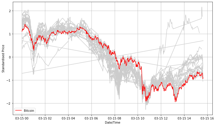
As the referral curve we made Bitcoin (in red) and the rest of series plotted in grey to spot a general pattern.
At the first glance it is obvious that not every cryptocurrency is so frequently traded as Bitcoin (notice gaps in price series). Interestingly, the trading direction is in a very good agreement with the Bitcoin pattern.
Let us now to transform the data to 1-min return series before moving forward.
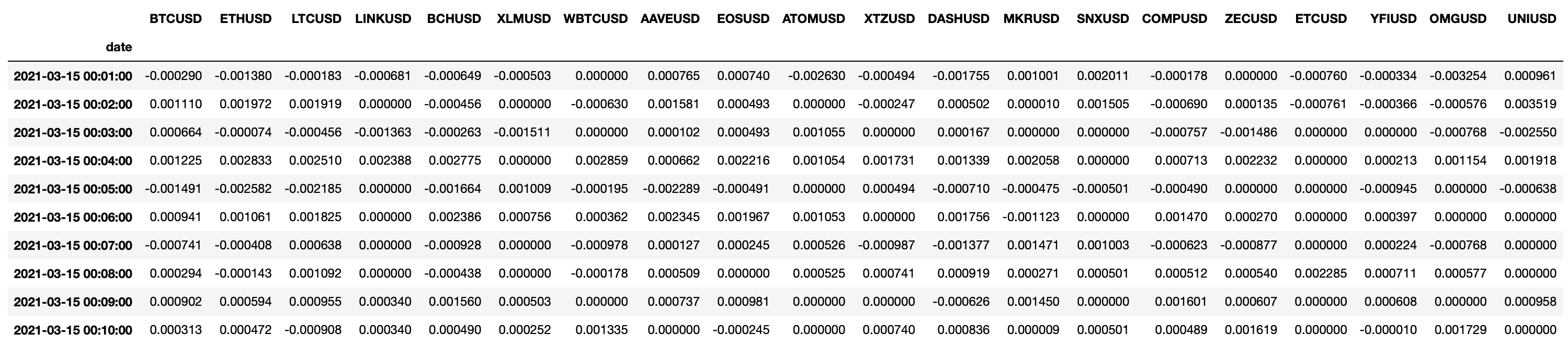
# data transformation
df_ret = df.pct_change(periods=1) # simple 1-min returns

# create and apply a 'NaN' mask
mask = df_ret.isna()
df_ret[mask] = np.nan

# remove all rows from DataFrame where all values are NaN
df_ret.dropna(how='all', axis=0, inplace=True)

del df_ret['GRTUSD']
del df_ret['ALGOUSD']
del df_ret['CGLDUSD']
del df_ret['UMAUSD']
The last step (getting rid of four assets) is performed based on manual inspection of return matrix. For these cryptocurrencies the number of zero 1-min returns was caused by the lack of sufficient data. Therefore, their inclusion in the core analysis made no sense.
2. Instantaneous Correlations
Let’s create a carbon copy of the return DataFrame which we will transform into directional return DataFrame object (df_ret_dir). At the beginning it will look like as expected:
df_ret_dir = df_ret.copy()

# display on the screen (Jupyter Notebook output)
display(df_ret_dir.head(10))
 Now, let’s apply the following data transformation :
for i in range(0, df_ret.shape[0]):
    row = df_ret.iloc[i]
    # determine BTCUSD direction of trading (-1 and +1)
    btc_sign = -1 if df_ret.iloc[i][0] < 0.0 else 1
    # rewrite the row
    df_ret_dir.iloc[i] = np.sign(row) == btc_sign  # apply boolean mask
This part is essential one. We move row by row of the DataFrame storing 1-min simple returns. For each row, we read out the value of the first cell which corresponds, of course, to the 1-min return of BTC/USD. If it is less than zero, we assign btc_sign as negative, otherwise as positive one. Next, we overwrite the entire row applying an operation of a sign comparison between a given coin’s return and the one of the Bitcoin.
Doing that way, for every timestamp, we extract an information whether a given asset was following the trading direction as displayed by Bitcoin or not. We might call it as the instantaneous correlation between crypto-returns vs Bitcoin.
In the end, we obtain df_ret_dir DataFrame transformed to the following form:
display(df_ret_dir.head(10))

3. Fraction of Crypto-Assets Instantaneously Correlated with Bitcoin
Given the results obtain above, we are just one step away from a determination of the fraction of crypto-assets instantaneously correlated with Bitcoin. It is sufficient if for every timestamp (row) of the df_ret_dir DataFrame we perform calculations as follows:
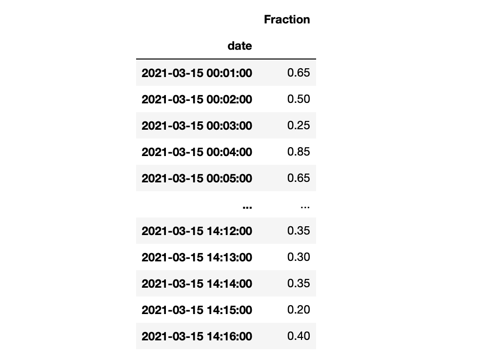
fraction = df_ret_dir.astype(int).sum(axis=1) / df_ret_dir.shape[1]

# visualise results
display(pd.DataFrame(fraction, columns=['Fraction']))
A cherry on the cake comes in the final chart:
fig, ax1 = plt.subplots(1,1, figsize=(12,9))

for ccy  in ret.columns.tolist():
    ax1.plot((df[ccy]-df[ccy].mean())/df[ccy].std(), color=grey)

ax1.plot((df['BTCUSD']-df['BTCUSD'].mean())/df['BTCUSD'].std(), 'r-', label='1-min BTCUSD')
ax1.grid()
ax1.set_ylabel('Normalised Price')
ax1.set_xlabel('Date and Time')
ax2 = ax1.twinx()
ax2.plot(ratio.iloc[1:], '-', color='#f09547', alpha=0.35, label='1-min Fraction')
ax2.plot(fraction.rolling(5).mean(), color='#f09547', label='5-min rolling average fraction')
ax2.set_ylabel('Fraction')
ax2.legend(loc=4)
ax1.legend(loc=3)
ax1.set_xlim([pd.to_datetime('2021-03-15 00:00'), pd.to_datetime('2021-03-15 13:00')])
plt.savefig("/Users/pawel/Desktop/trig6.png", bbox_inches='tight')
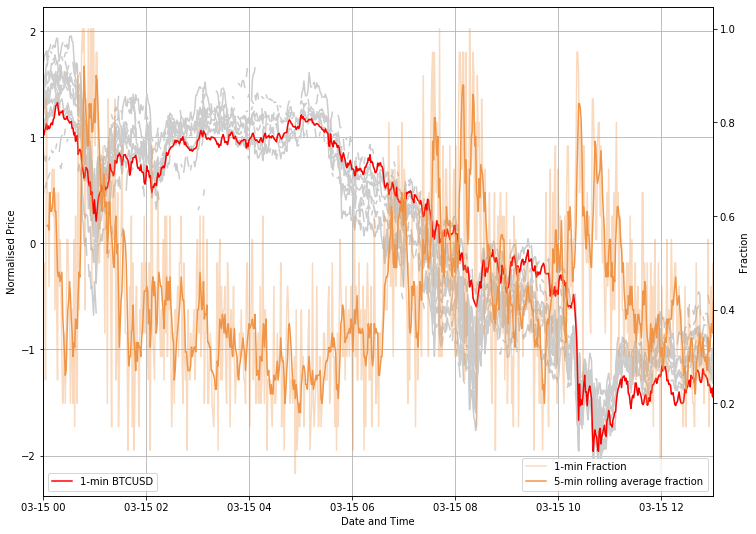
This reveals quite spectacular state of the drama during sudden Bitcoin sell-offs. The fraction of assets following BTC may be as high as 95% or even 100% in certain minutes of trading (see pale orange curve). The 5-min rolling mean of computed fractions can be, therefore, used as a lagged sell-off risk measure. This, of course, remains valid under a silent assumption we made here, i.e. that Bitcoin leads the horde of crypto-buddies.
An optical zoom onto the fall at 10:20 of March 15, 2021 as underlined by 3-min rolling average fraction:
fig, ax1 = plt.subplots(1,1, figsize=(12,7))

for ccy  in ret.columns.tolist():
    ax1.plot((df[ccy]-df[ccy].mean())/df[ccy].std(), color=grey)

ax1.plot((df['BTCUSD']-df['BTCUSD'].mean())/df['BTCUSD'].std(), 'r-', label='1-min BTCUSD')
ax1.grid()
ax1.set_ylabel('Normalised Price')
ax1.set_xlabel('Date and Time')
ax2 = ax1.twinx()
#ax2.plot(ratio.iloc[1:], '-')
ax2.plot(fraction.rolling(3).mean(), color='#f09547', label='3-min rolling average ratio')
ax2.set_ylabel('Fraction')
ax2.legend(loc=1)
ax1.legend(loc=3)
ax1.set_ylim([-2.1, 0])
ax1.set_xlim([pd.to_datetime('2021-03-15 08:30'), pd.to_datetime('2021-03-15 13:00')])
plt.title('Max Fraction = %.1f%% at %s' %
          (100*(fraction[fraction.index > '2021-03-15 08:30']).max(),
           fraction[fraction.index > '2021-03-15 08:30'].index[fraction[fraction.index >
                                                               '2021-03-15 08:30'].argmax()]))
shows that 95% of assets were (or could be!) simultaneously dragged down by the Bitcoin itself:
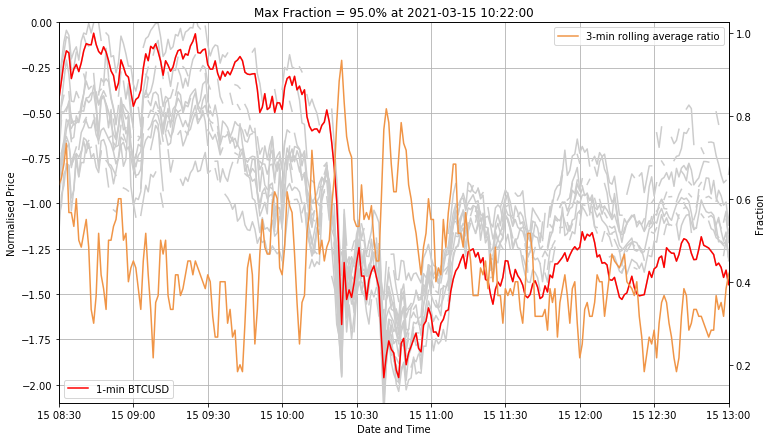
The most likely explanation of this coherent movements one may link to high-frequency trading algorithms following the price movements in BTC/XXX space and reacting on the time-scales shorter than 60 seconds.
As a homework you might re-use the same code to find out whether Bitcoin may also co-lead upward price movements and how frequently that happens in comparison to these short-term Bitcoin sell-offs.